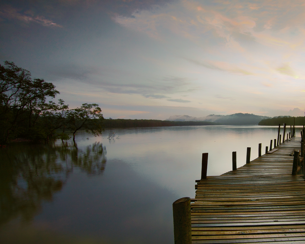
[CGDI] Color Transfer via Discrete Optimal Transport using the *sliced* approach == > [name="David Coeurjolly"] ENS [CGDI](https://perso.liris.cnrs.fr/vincent.nivoliers/cgdi/) Version [TOC] --- Color transfer is an image processing application where you want to retarget the color histogram of an input image according to the color histogram of a target one. **Example:** Input image | Target image | Color transfer output -------|---------|---- 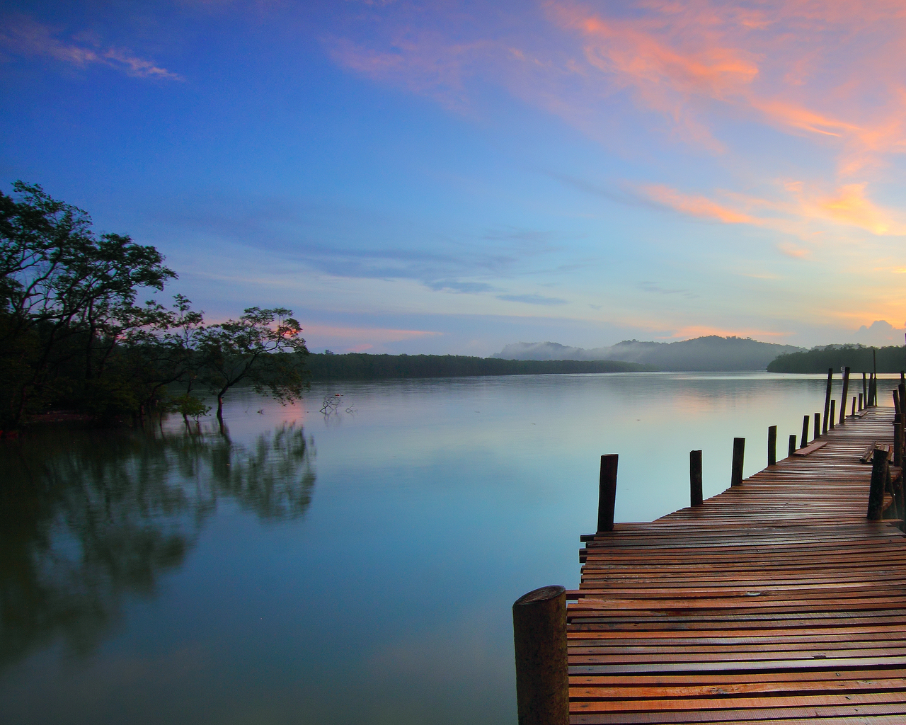 | 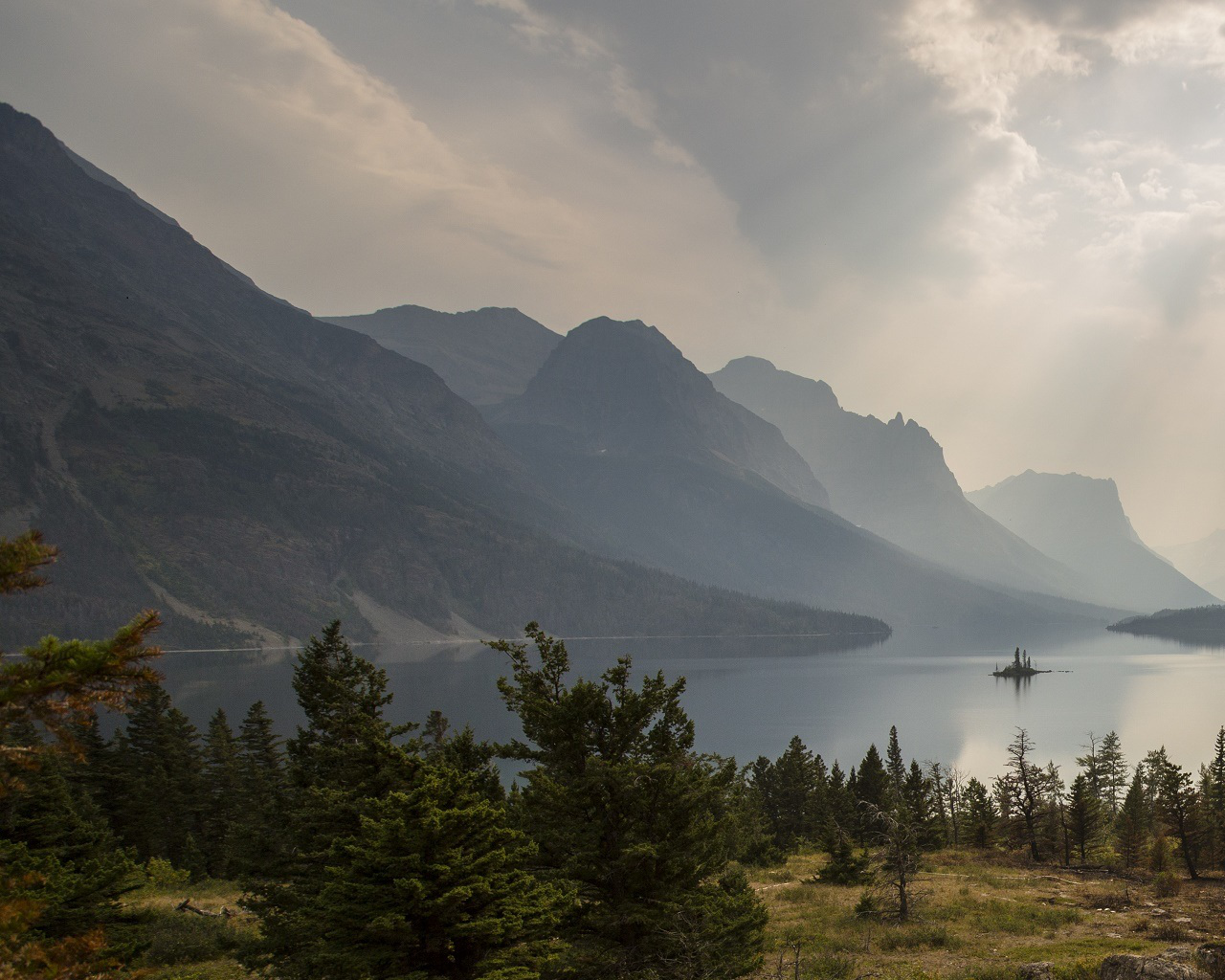 |  The idea of this project is to detail a color transfer solution that considers the [Optimal Transport](https://en.wikipedia.org/wiki/Transportation_theory_(mathematics)) as a way to *deform* histograms in the most *efficient way* (see below for details). The objective of this TP is to implement a *sliced* approach to solve the color transfer problem via Optimal Transport. # Warm-up 1: Downloading the code The skeleton of the code is available on [this Github Project](https://github.com/dcoeurjo/CGDI-Practicals). This code contains all you need to load and save color images (and to parse command line parameters for the `c++`code). You can download the archive from the Github interface (*"download zip"* menu), or *clone* the git repository. The project contains some `c++` and `python` codes. :::warning For python, we encourage you to use the notebooks shared by Vincent on the [CGDI homepage](https://perso.liris.cnrs.fr/vincent.nivoliers/cgdi/). ::: To compile the C++ tools, you would need [cmake](http://cmake.org) (>=3.14) to generate the project. For instance on linux/macOS: ``` bash git clone https://github.com/dcoeurjo/CGDI-Practicals cd CGDI-Practicals mkdir build ; cd build cmake .. -DCMAKE_BUILD_TYPE=Release make ``` On Windows, use cmake to generate a Visual Studio project. The practical work described below can be done either in `c++` or `python`. In the next section, we briefly introduce Optimal Transport and Sliced Optimal Transport (you can skip this section if you have followed the lecture). # Warm-up 2: Elementary Histogram Processing Either in `c++` and `python`, implement several basic histogram processing tools you have already discussed in the lecture: 1. RGB -> Grayscale transform: Just convert a color image to a single channel grayscle one. 2. [Gamma correction](https://en.wikipedia.org/wiki/Gamma_correction) (each channel of the RGB images will be processed independently). # Brief overview:  Optimal Transport and Sliced Optimal Transport As mentioned above, the key tool will be Optimal Transport (OT for short) which can be sketched as follows: Given two probability (Radon) measures $\mu\in X$ and $\nu\in Y$, and a *cost function* $c(\cdot,\cdot): X\times Y \rightarrow \mathbb{R}^+$, an optimal transport plan $T: X\rightarrow Y$ minimizes $${\displaystyle \inf \left\{\left.\int _{X}c(x,T(x))\,\mathrm {d} \mu (x)\;\right|\;T_{*}(\mu )=\nu \right\}.}$$ The cost of the optimal transport defines a metric between Radon measure. We can define the $p^{th}$ [Wasserstein metric](https://en.wikipedia.org/wiki/Wasserstein_metric), $\mathcal{W}_p(\mu,\nu)$ as $$\displaystyle \mathcal{W}_{p}(\mu ,\nu ):={\left(\displaystyle \inf \left\{\left.\int _{X}c(x,T(x))^p\,\mathrm {d} \mu (x)\;\right|\;T_{*}(\mu )=\nu \right\}\right)^{1/p}}$$ An analogy with piles of sand is usually used to explain the definition: let us consider that $\mu$ is a pile of sand and $\nu$ a hole (with the same *volume* or *mass*), if we consider that the cost of moving an elementary volume of sand from on point to the other is proportional to the Euclidean distance ($l_2$ cost function), then the optimal transport plan gives you the most efficient way to move all the sand from $\mu$ to $\nu$. Again, the literature is huge and there are many alternative definitions, please refer to [Computational Optimal Transport](https://optimaltransport.github.io/book/) for a more complete introduction to the subject. The link between OT and color transfer follows the observation that color histograms are discrete Radon measures. As we are looking for the *most efficient* transformation of the input image histogram to match with the target one, the color transfer problem can be reformulated as a discrete OT one [^b1][^b2][^b2b][^b3][^b4][^b5]. 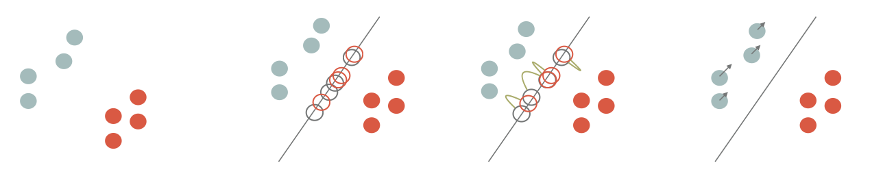There are many numerical solutions to compute the OT (with continuous, discrete, semi-discrete measures, w/o regularization...). We focus here on the **sliced** formulation of the OT and associated 2-Wasserstein metric in dimension $d$: $$ SW^2_2(\mu,\nu) := \int_{\mathbb{S}^d} \mathcal{W}_2^2( P_{\theta,\sharp}\mu,P_{\theta,\sharp}\nu) d\theta\,.$$ The sliced formulation consists in projecting the measures onto a 1D line ($P_{\theta,\sharp}: \mathbb{R}^d\rightarrow \mathbb{R}$), solving the 1D OT problem on the projections and average the results for all directions ($\mathbb{S}^d$ is the unit hypersphere in dimension $d$). If the measures are discrete as the sums of Diracs centered at points $\{x_i\}$ and $\{y_i\}$ in $\mathbb{R}^d$ ($\mu := \frac{1}{n}\sum_{x_i} \delta_{x_i}$, $\nu := \frac{1}{n}\sum_{y_i} \delta_{y_i}$), then the 1D OT is obtained by sorting the projections and computing the difference between the first projected point of $\mu$ with the first projected point of $\nu$, the second with the second, etc... $$ SW^2_2(\mu,\nu) = \int_{\mathbb{S}^d} \left(|\langle x_{\sigma_\theta(i)} - y_{\kappa_\theta(i)},\theta\rangle|^2 \right) d\theta\,,$$ ($\sigma_\theta(i)$ a,d ${\kappa_\theta(i)}$ are permutations with increasing order). Numerically, we sample the set of directions $\mathbb{S}^d$ and thus consider a finite number of *slices*. # Sliced OT Color Transfer, the "TP" Back to our histogram transfer problem, Diracs centers $\{x_i\}$ are points in RGB space (one Dirac per pixel of the input image), and $\{y_i\}$ are the colors of the target image. Matching the histogram can be seen a transportation of the point cloud $\mu$ to $\nu$ in $\mathbb{R^3}$ (the RGB color space). The idea is to advect points of $\mu$ such that we minimize $SW(\mu,\nu)$. As described in the literature[^b1][^b2b][^b4], this amounts to project he points onto a random direction $\theta$, *align* the sorted projections and advect $\mu$ in the $\theta$ direction by $|\langle x_{\sigma_\theta(i)} - y_{\kappa_\theta(i)},\theta\rangle|$.  ### The core 3. Get the `C++` / `python`. In Both cases, we provide elementary code to load/save RGB images. Please check how to access to RGB pixel values. 2. Create a function to draw a random direction ::: info **Info**: to uniformly sample a direction in $\mathbb{R}^d$, a classical approach is to draw a $d$ dimensional random vector where each component follows a normal distribution (e.g. using C++ `std::normal_distribution`), with mean 0 and standard deviation equal to 1.0. Then normalize the vector and you have a uniform sampling of $\mathbb{S}^d$. ::: 3. From now on, the source (or target) image will be seen as a 3d point cloud in RGB space. Create a function to sort the projection of the samples of one image onto a random direction. :::info **Tip**: consider using a custom sort predicate in the C++ `std::sort` function. ::: 4. On this random direction $\theta$, sort both sample sets (source and target one) and advect the first sample, denoted $p_i$, of the source, along the $\theta$ direction, by an amount $d$ which correspond to the difference between projection of this first source sample, and the projection of the first target sample. In other words: $$\vec{Op_i} = \vec{Op_i} + \langle x_{\sigma_\theta(0)} - y_{\kappa_\theta(0)},{\theta}\rangle ~{\theta}\,.$$ Do the same for the second ones, and the remaining samples. :::info **Tip**: Be careful when performing some computations on RGB `unsigned char` values. A good move would be to convert all data to `double` from the very beginning (and convert them back to `unsigned char` before exporting). ::: 5. Implement the main loop of the sliced approach: repeat the steps (draw a direction, sort the projections, compute the displacements, advect the source sample) until a maximum number of steps is reached. 6. To better set the maximum number of slices, output the sliced optimal transport energy with respect to the number of slices. You should also be able to *visualize* the convergence: {%youtube FiVPXl3Io0w%} ### Advanced features 7. **Batches.** Instead of advecting $\mu$ for each $\theta$, we can accumulate advection vectors into a small batch and perform the transport step once the batch is full[^b4]. This corresponds to a stochastic gradient descent strategy in ML. Implement this "batch" approach. Compare this approach w.r.t to the legacy one (in terms of speed of convergence for instance). 8. **Regularization.** To obtain a smoother result or to be able to handle noise in the inputs, a classical approach consists in considering *regularized* optimal transport, or to regularize the optimal transport plan at the end of the computation. For color transfer, a simple way to mimic this approach consists in applying a non-linear smoothing filter to the transport plan[^b4]. A way to achieve this is to: * once the sliced approach has converged, let's say we have a transformed source image $S^*$ of the image $S$ w.r.t. the target $T$; * we express the transport plan as an *image* $(S^*-S)$; * we can filter this image (using for instance a [bilateral filter](https://en.wikipedia.org/wiki/Bilateral_filter)) to obtain the final image : $\tilde{~S} = S + filter_\sigma(S^*-S)$. :::info **Tip**: In the `c++` project, we have included the [cimg](https://cimg.eu) header which contains an implementation of the bilateral filter. On `python`, the [OpenCV](https://opencv.org) package has been imported (which also contains an implementation of the bilateral filter). ::: 9. **Interpolation**: One can mimic the interpolation between two discrete measures in the sliced formulation by simply tweaking the advection step: instead of computing $\vec{Op_i} = \vec{Op_i} + \langle x_{\sigma_\theta(0)} - y_{\kappa_\theta(0)},{\theta}\rangle ~{\theta}$, just compute $\vec{Op_i} = \vec{Op_i} + \alpha\langle x_{\sigma_\theta(0)} - y_{\kappa_\theta(0)},{\theta}\rangle ~{\theta}$ for some $\alpha\in[0,1]$. You should be able to obtain something like that: {%youtube Ti6kjJSdRnA%} 10. **Partial optimal transport**: as you may have noticed, the source and target images **must** have the same number of pixels. When the two discrete measures do not have the same number of Diracs, we are facing a *partial* optimal transport problem[^b6] (the overall all *sliced* approach remains the same, the 1D OT problem along the direcrtion is slightly more complicated). Without going to this *exact* partial solution, could you imagine and implement an approximate solution that *does the job* when the two images do not have the same size? # References [^b1]: Francois Pitié, Anil C. Kokaram, and Rozenn Dahyot. 2005. N-Dimensional Probablility Density Function Transfer and Its Application to Colour Transfer. In Proceedings of the Tenth IEEE International Conference on Computer Vision - Volume 2 (ICCV ’05). IEEE Computer Society, Washington, DC, USA, 1434–1439. https://doi.org/10.1109/ ICCV.2005.166 [^b2]: François Pitié, Anil C Kokaram, and Rozenn Dahyot. 2007. Automated colour grading using colour distribution transfer. Computer Vision and Image Understanding 107, 1-2 (2007), 123–137. [^b2b]: Rabin Julien, Gabriel Peyré, Julie Delon, Bernot Marc, Wasserstein Barycenter and its Application to Texture Mixing. SSVM’11, 2011, Israel. pp.435-446. hal-00476064 [^b3]: Nicolas Bonneel, Julien Rabin, G. Peyré, and Hanspeter Pfister. 2015. Sliced and Radon Wasserstein Barycenters of Measures. J. of Mathematical Imaging and Vision 51, 1 (2015). [^b4]: Julien Rabin, Julie Delon, and Yann Gousseau. 2010. Regularization of transportation maps for color and contrast transfer. In Image Processing (ICIP), 2010 17th IEEE International Conference on. IEEE, 1933–1936. [^b5]: Nicolas Bonneel, Kalyan Sunkavalli, Sylvain Paris, and Hanspeter Pfister. 2013. Example- Based Video Color Grading. ACM Trans. Graph. (SIGGRAPH) 32, 4 (2013). [^b6]: Nicolas Bonneel and David Coeurjolly. 2019. Sliced Partial Optimal Transport. ACM Trans. Graph. (SIGGRAPH) 38, 4 (2019).