---
title: IPCV Practical - Geometric estimations on 3d digital surfaces
---
IPCV Practical - Geometric estimations on 3d digital surfaces
===
> [name=Jacques-Olivier Lachaud][time=Oct 2022][color=#907bf7]
###### tags: `DGtal` `3d`
[TOC]
The objective of this practical is to compute a few geometric quantities on digital surfaces and compare them with ground truth values using [DGtal](https://dgtal.org). It also highlights the asymptotic relations of a smooth Euclidean shape with its digitized counterpart.
## Getting started
In the DGtal-DGMM `practical-3D-estimation` repository, have a look to the `3D-estimation.cpp` file. If you are in your build repository, it should compile as is and is executed simply in the command line with
```
./3D-estimation
```
You may choose your implicit shape and digitization step. The program computes the digital surface in-between interior/exterior points, then convert it to a polygonal quad mesh called *primal surface*. It is its natural digital embedding as the boundary of a union of voxels.
| sphere9 $h=0.5$ | torus $h=0.5$ | torus $h=0.25$ |
| -------- | -------- | -------- |
| 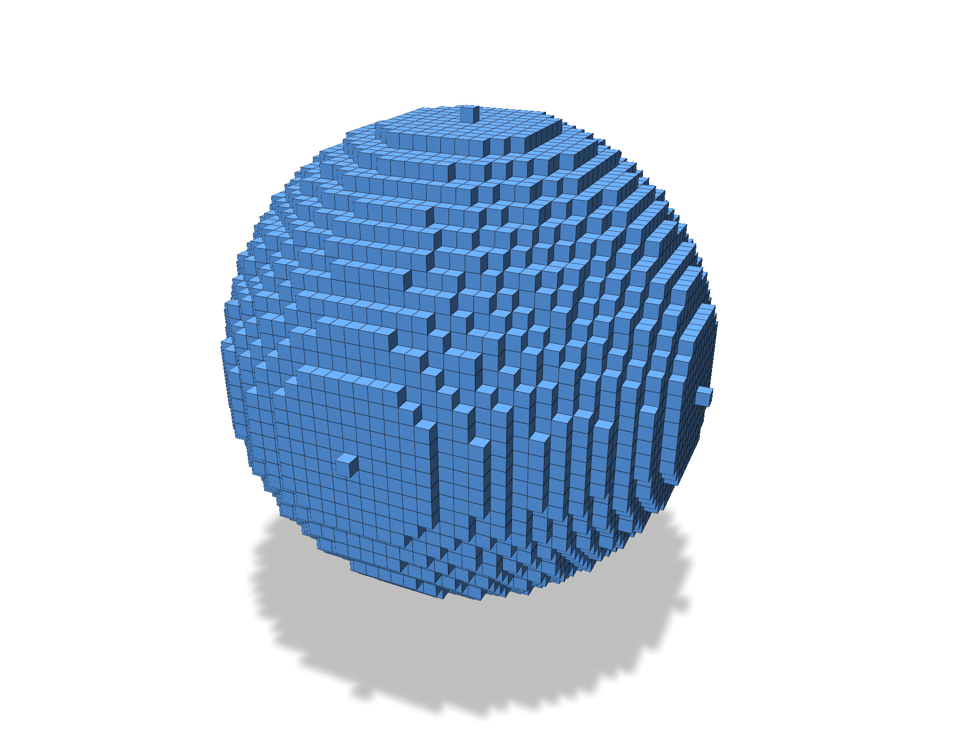 |  | 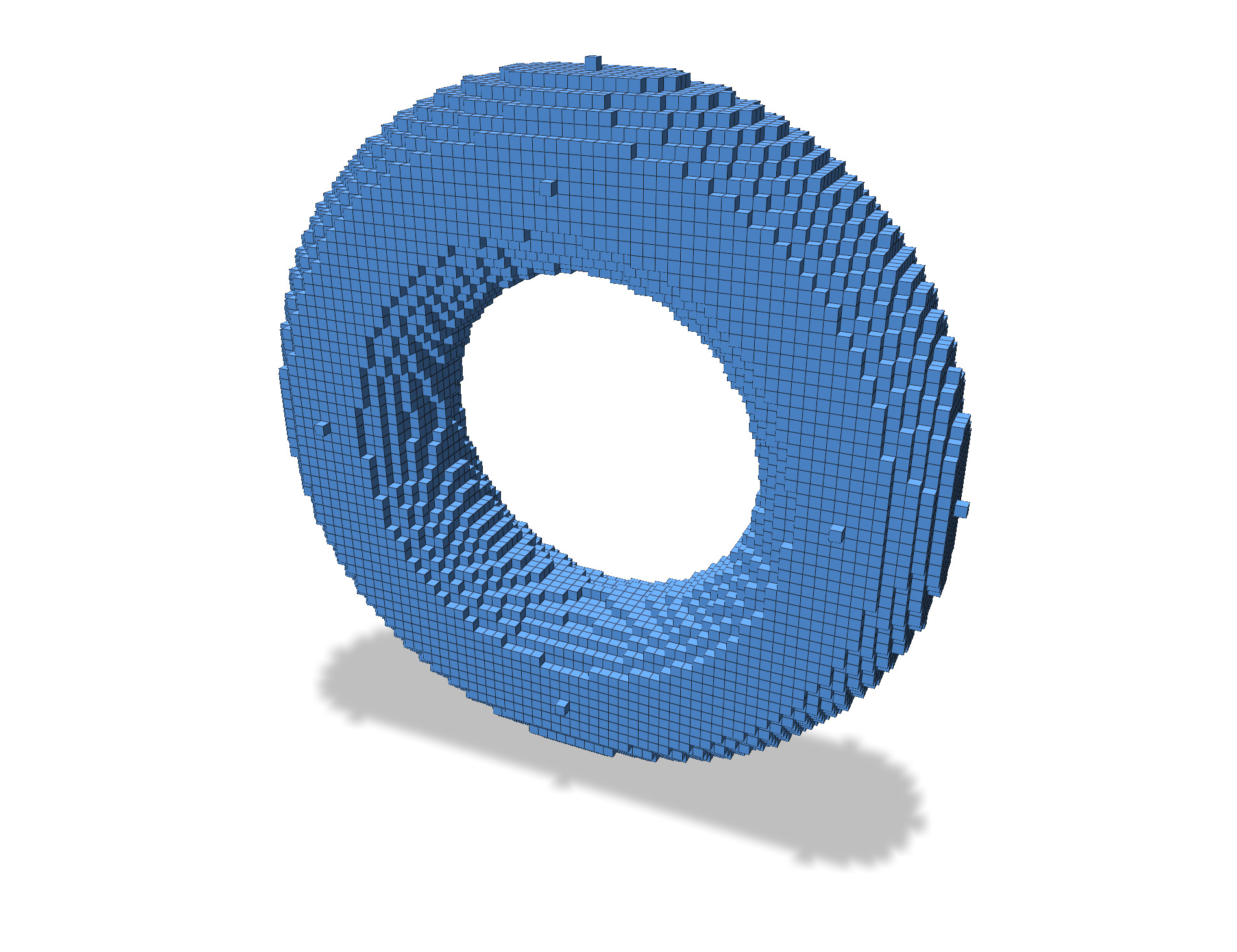|
:::danger
:::spoiler Performances
When you code is up and running on small volumetric files, make sure to compile the project in cmake `Release` mode to get best performances (internal asserts will be disabled).
:::
:::success
:::spoiler Primal surface?
The primal surface of a digital object corresponds to an embedding of the [digital surface](https://dgtal-team.github.io/doc-nightly/moduleDigitalSurfaces.html) (boundary of the union of the voxels) in the [Khalimsky grid](https://dgtal-team.github.io/doc-nightly/moduleCellularTopology.html), to the Euclidean space. I.e. 2-cells (cells of dimension 2 of the Khalimsky complex) corresponding to the boundary between interior and exterior voxels are embedded as unit squares.
:::
:::info
:::spoiler **Exercise** : add new shapes
You may start your practical by adding a few implicitly defined shapes to the program. "goursat", "leopold", "goursat-hole" are popular examples. Expect one line of code per shape.
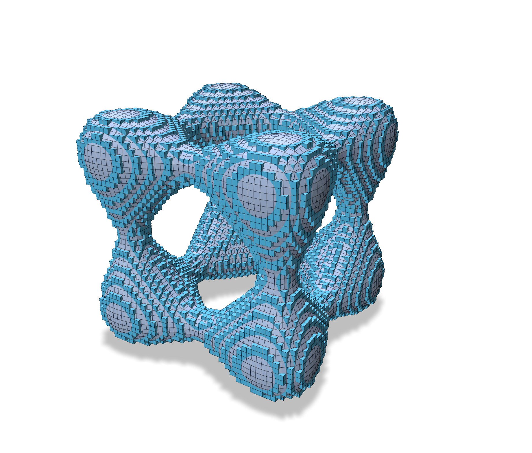
| goursat $h=0.25$ | leopold $h=0.25$ | goursat hole $h=0.25$ |
| -------- | -------- | -------- |
| 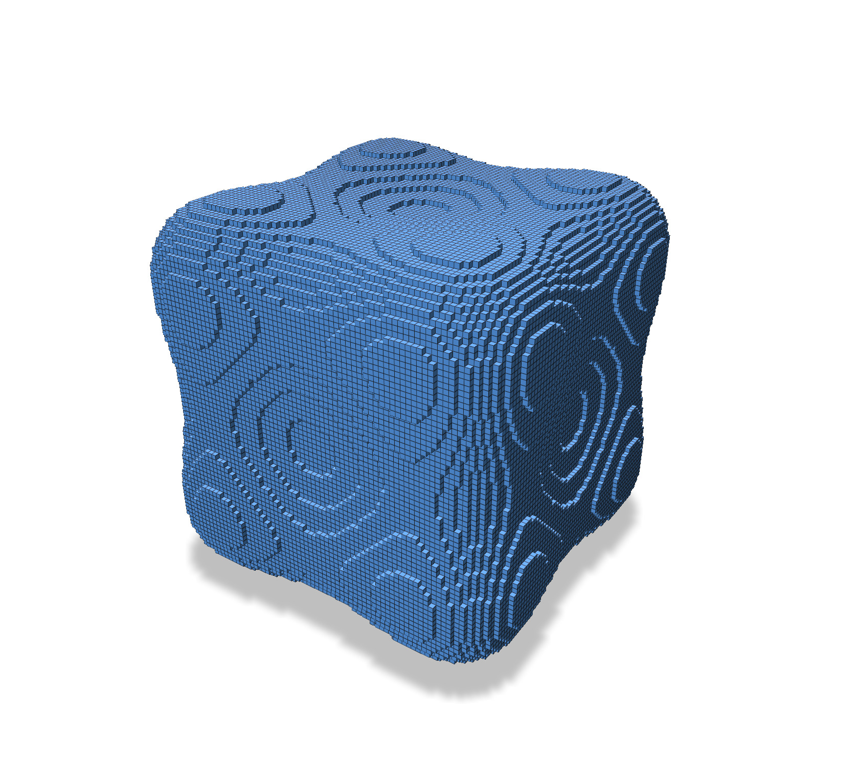 | 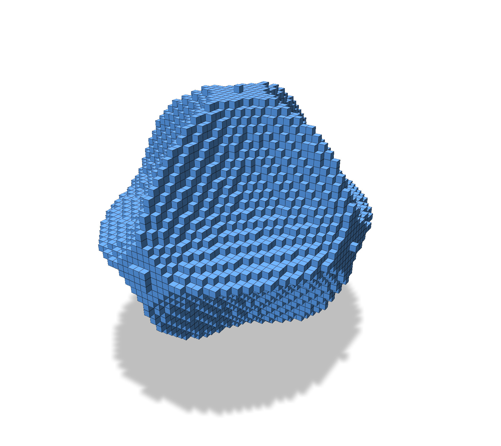 | 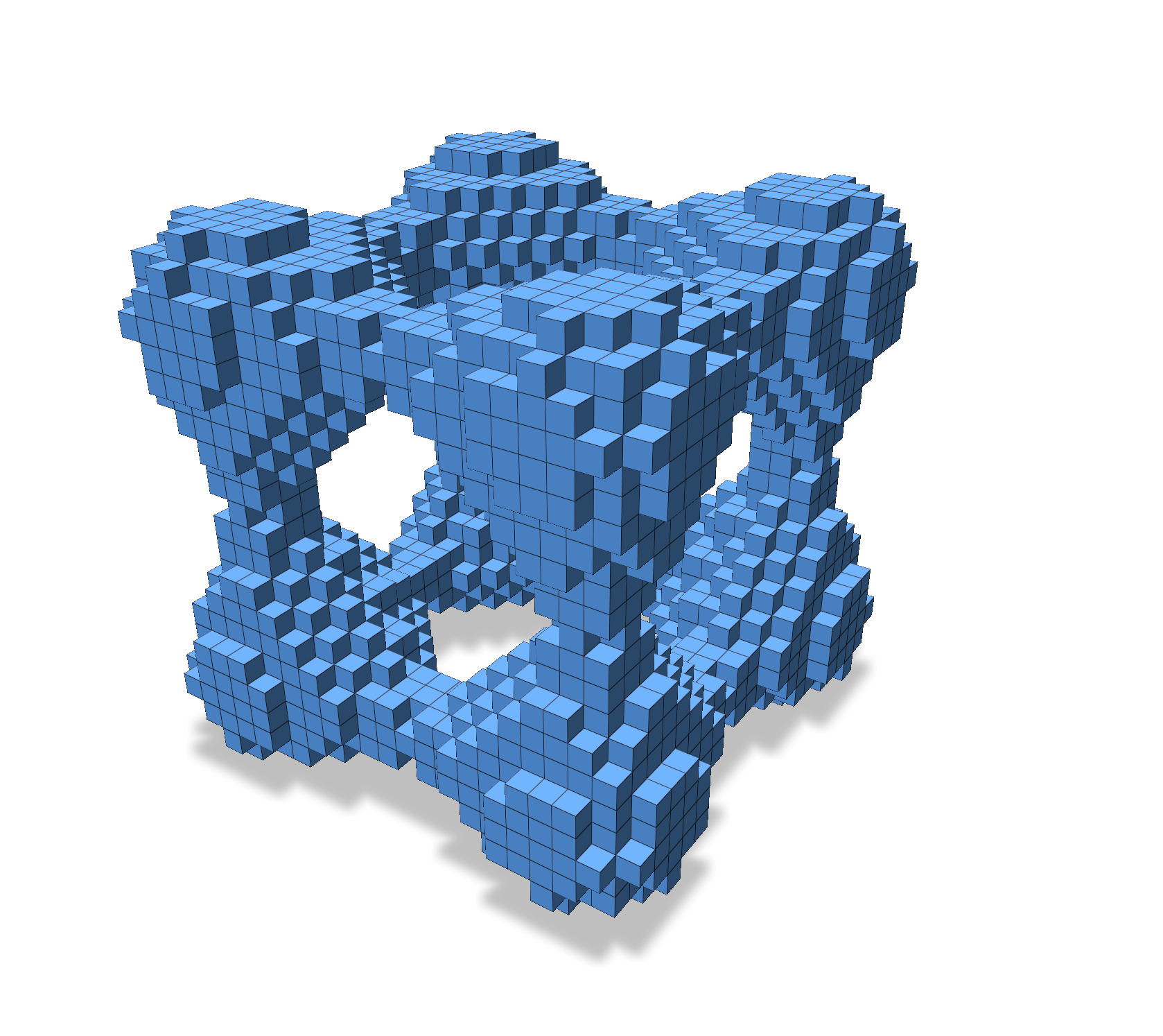 |
:::
## 3D geometric estimations
This section shows how to estimate correctly the area of a digital object. We start by estimating a normal vector field on the surface, and then the global area is estimated through local computations.
The main part of the documentation for this practical is the one related to [shorcuts](https://dgtal-team.github.io/doc-nightly/moduleShortcuts.html). It provides you a lot of ready-to-use functions to load/build volume and surfaces, computes some geometric quantities, and export them.
:::success
:::spoiler Philosophy of [shorcuts](https://dgtal-team.github.io/doc-nightly/moduleShortcuts.html) module
This module hides as many as possible implementations details when dealing with digital and mesh surfaces. You pass with a `Parameter` object many informations to shorcuts. You specify the shape, the digitization gridstep, the radius parameter of an estimator, the chosen topology, which connected component you want, etc. The module also chooses what kind of digital surface you use.
`C++11` is very convenient with the `auto` keyword, which lets you largely ignore what object you are manipulating.
:::
### Getting a normal vector field onto a digital surface
[shorcuts](https://dgtal-team.github.io/doc-nightly/moduleShortcuts.html) offers you several ways to compute a normal vector field onto the whole digital surface or onto a part of it.
You can already view the "true" normal vector field of the implicit surface. It was computed and displayed with these two lines
```cpp
auto true_normals = SHG3::getNormalVectors( shape, K, surfels, params );
psMesh->addFaceVectorQuantity( "True normal vector field", true_normals );
```
There are several normal vector fields that are computable by shorcuts (see [philosophy of shorcuts module](https://dgtal-team.github.io/doc-nightly/moduleShortcuts.html#dgtal_shortcuts_sec3)):
- `ShortcutsGeometry::getTrivialNormalVectors`: returns the trivial (T) normal vectors to the given surfel range
- `ShortcutsGeometry::getCTrivialNormalVectors`: returns the convolved trivial (CT) normal vectors to the given surfel range
- `ShortcutsGeometry::getVCMNormalVectors`: returns the Voronoi Covariance Measure (VCM) normal vectors to the given surfel range
- `ShortcutsGeometry::getIINormalVectors`: returns the Integral Invariant (II) normal vectors to the given surfel range (embedded in a binary image or a digitized implicit shape)
Some of these methods are influenced by the `Parameter` object. However, they have default reasonnable values.
:::info
:::spoiler **Exercise** : add computation of several normal vector fields
You can for instance add the computation of the trivial (T), the convolved trivial (CT) and integral invariant (II) normal estimator. If you wish to let the user choose, you can use `ImGui::RadioButton`.
```cpp
int Estimator;
...
ImGui::RadioButton("Method 0", &Estimator, 0); ImGui::SameLine();
ImGui::RadioButton("Method 1", &Estimator, 1); ImGui::SameLine();
ImGui::RadioButton("Method 2", &Estimator, 2);
```
| (T) vector field of sphere $h=1$ | (II) vector field of sphere $h=1$|
| -------- | -------- |
| 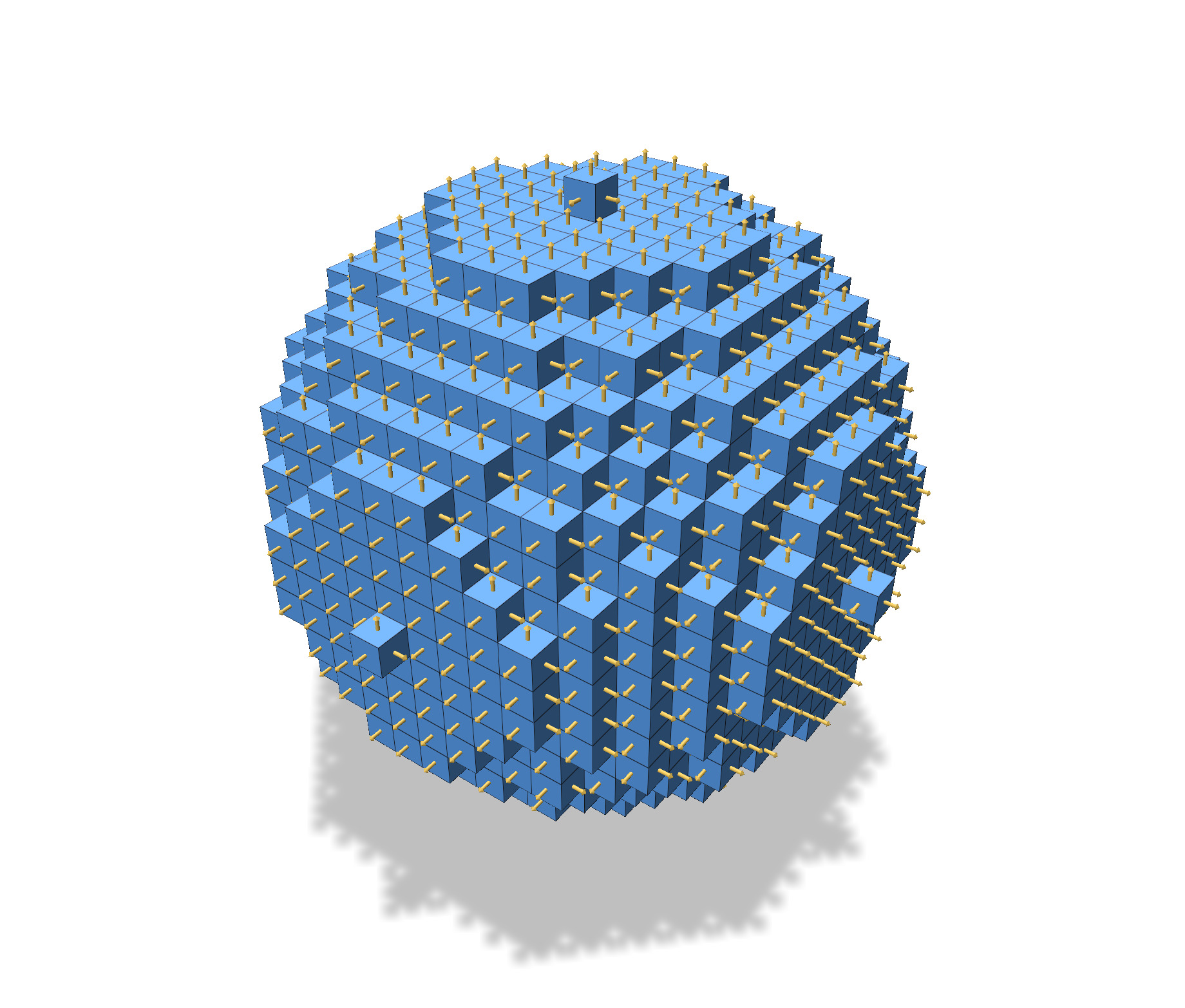 | 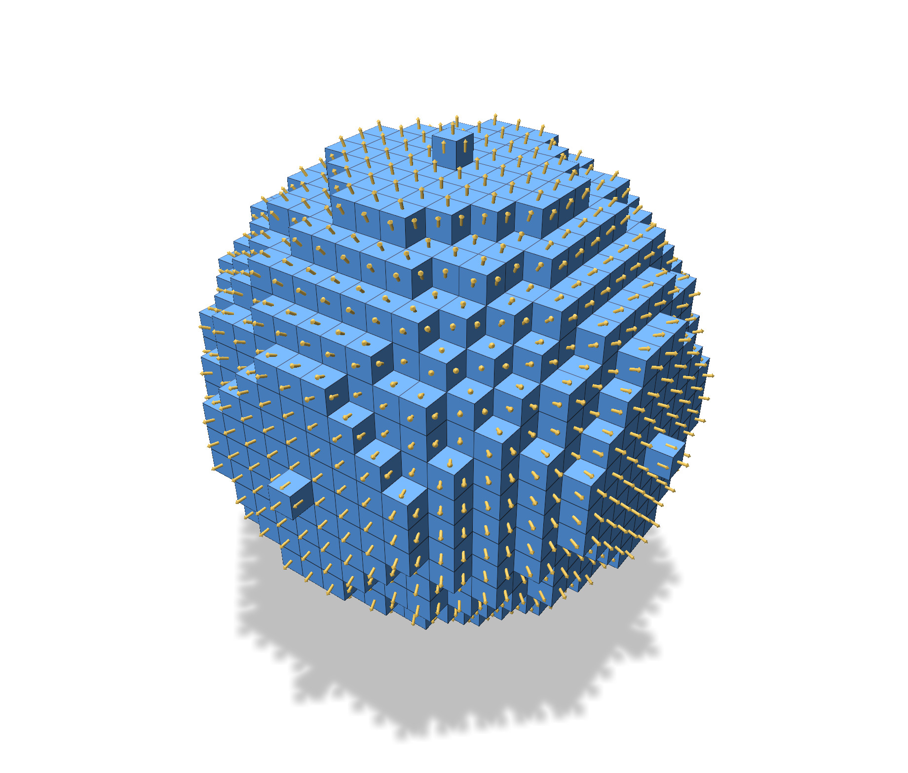 |
:::
:::info
:::spoiler **Exercise (optional)** : view errors in normal estimation
[shorcuts](https://dgtal-team.github.io/doc-nightly/moduleShortcuts.html#dgtal_shortcuts_sec3) provides you method to compute the angle error between two unit vector field. You may observe where the angle error is big by adding a face scalar quantity to your mesh:
```cpp
psMesh->addFaceScalarQuantity( "Angle error", angle_diff )
->setMapRange( { 0.0, M_PI / 20.0 } ) // 10° is bad !
->setColorMap( "coolwarm" );
```
| (T) angle error of sphere $h=1$ | (II) angle error of sphere $h=1$ |
| --------------- | -------- |
| | 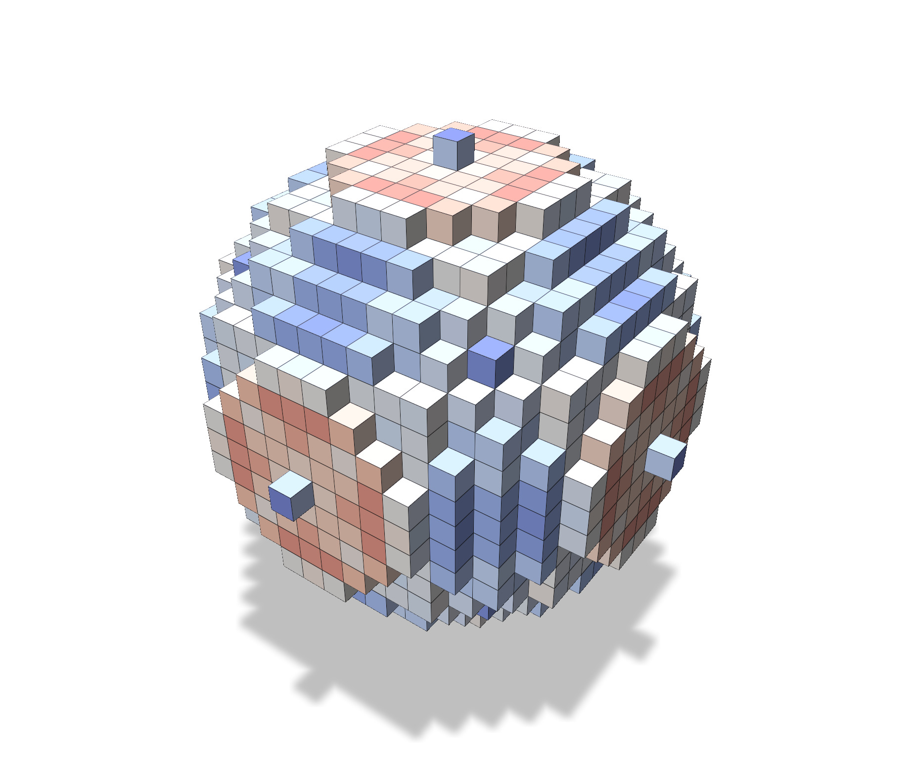 |
:::
:::info
:::spoiler **Exercise (optional)** : compute $l_2$ and $l_\infty$ errors in normal estimation
You can also compute the $l_\infty$-error of normal vector estimation, by computing the maximum of angle errors. For the $l_2$-error, the easiest way is to compute the squared root of the variance of angle errors. Use `ShorcutsGeometry::getStatistic` to get a statistic object from your vector of angle errors.
For the `sphere9` object, you would get something like:
| sphere9 | $l_\infty$-error (T) | $l_\infty$-error (CT) | $l_\infty$-error (II) |
| ------- | -------------------- | --------------------- | --------------------- |
| $h=1$ | 1.516 | 0.141 | 0.139 |
| $h=0.5$ | 1.543 | 0.190 | 0.077 |
| $h=0.25$| 1.557 | 0.183 | 0.041 |
Only the (II) estimator looks multigrid convergent.
:::
### Two methods for estimating the area
We propose two methods for computing the area, both of them works with local summations involving normal vectors. Let $\mathbf{X}$ be the smooth implicit shape, $\mathbf{X}_h$ its Gauss digitization at step $h$. Let us denote $(\mathbf{t}_i)$ the trivial normal vectors for each surfel $i$, and $(\mathbf{u}_i)$ any one of your estimated normal vector field. We will also use $(\mathbf{n}_i)$ as the exact normal vector field (it is the true normal of the implicit surface at the nearest point to the surfel centroid).
1. The first method, sometimes called Euler integration, takes the scalar product of the trivial normal with the estimated normal (formula related to classical integration change of variables):
$$
\widehat{\mathrm{Area}_1}(\mathbf{X}_h,h) := h^2 \sum_{\text{surfels}~i~\text{of}~X_h} \mathbf{t}_i \cdot \mathbf{u}_i.
$$
2. The second method, proposed in [^6], takes the inverse of the $l_1$-norm of each estimated normal vector (formula related more to a statiscal analysis of digital planes):
$$
\widehat{\mathrm{Area}_2}(\mathbf{X}_h,h) := h^2 \sum_{\text{surfels}~i~\text{of}~X_h} \frac{1}{\|\mathbf{u}_i\|_1}.
$$
:::info
:::spoiler **Exercise**: Compute the estimated area using both methods
Use the formulas above and your normal vector fields to perform the area estimations. You may display the result in your GUI with something like:
```cpp
ImGui::Text( "Area1=%f Area2=%f", Area1, Area2 );
```
For a sphere of radius $r$, the true area is $4 \pi r^2$, hence for `sphere9`, expect $1017.87601976309300925456$.
:::
### Checking the multigrid convergence
A natural question is if these area estimates tends to the area of the Euclidean shape as the digitization gets finer and finer, aka are your area estimators **multigrid convergent** [^3] ?
:::success
For Euler integration method (method 1), Theorem 4 [^5] asserts that $\widehat{\mathrm{Area}_1}$ estimator is multigrid convergent as long as the estimated normal vector field $\mathbf{u}$ is itself convergent. The worst-case speed is then of the same order.
Convergence of (II) normal vector field is proven in [^1] and its speed of convergence is explicited in [^4]. Convergence of (VCM) normal vector field is proven in [^2].
:::
:::warning
For method 2, it has been solely proven for the digitization of a plane. It is conjectured to be true too.
:::
Let us find out if any our area estimators are indeed experimentally convergent. What speed of convergence do we get in practice ?
:::info
:::spoiler **Exercise**: compute areas for a sequence of shapes with finer and finer digitization.
You may either use your GUI to compute by hand each error, or creates a new button that launches these computations, without creating a shape in the polyscope interface (copy/paste is your friend).
For a sphere object, you have easily the true area $A$, so the relative error is computed as $\left|\frac{\widehat{\mathrm{Area}_k}(\mathbf{X}_h,h)-A}{A}\right|$.
For other shapes, you can have an idea of the convergence by using the area estimator with the true normal vector field $\mathbf{n}$. In some sense, you cannot expect a better result at the given resolution.
The table below displays the relative error for method 1 (Euler Integration):
| `sphere9` | $\mathbf{u}=$(T) | $\mathbf{u}=$(CT) | $\mathbf{u}=$(II) |
| --------- | ---------------- | ----------------- | ----------------- |
| $h=1$ | $49.134$% | $3.200$% | $0.369$% |
| $h=0.5$ | $48.692$% | $5.469$% | $0.335$% |
| $h=0.25$ | $49.319$% | $4.645$% | $0.105$% |
| $h=0.125$ | ... | | |
- Is method 1 before than method 2 ?
- What is the speed of convergence (hint: display graph with gnuplot in logscale) ?
:::
## Going further: properties of digitized shapes
The purpose now is to analyze more closely the relations between the smooth object and its digitization. Especially we want to relate the surface $\partial \mathbf{X}$ of the smooth shape $\mathbf{X}$ to the boundary $\partial \mathbf{X}_h$ of the digitized shape $\mathbf{X}_h := \mathbf{X} \cap h\mathbf{Z}^d$ (Gauss digitization).
As detailed in [^5], most of the properties are related to the **reach** of $\partial \mathbf{X}$, which is the infimum of its distances to the medial axis. The reach is related to the curvatures of $\partial \mathbf{X}$, and cannot exceed the inverse of the largest principal curvature in absolute value. For instance the reach of the sphere with radius $r$ is $r$ itself.
We will see that a digitized boundary is always close to its smooth counterpart. However, even for very smooth shapes, the digitized boundary is not in general a 2-manifold in the continuous sense (however, it is indeed a digital surface, but you add specific connectedness to resolve the non-manifold places). We will also see that the ambient **projection** $\pi$ onto the shape boundary $\partial \mathbf{X}$ is not everywhere 1-1 map.
### Proximity between smooth and digitized boundary
It is very easy to get an approximation of the smooth surface. It is obtained by just projecting the vertices of the digitized surface onto the level zero of the implicit shape (using a gradient descent). `ShorcutsGeometry::getPositions` does the job.
:::info
:::spoiler **Exercise**: Compute the smooth surface and display it.
```cpp
auto ppositions = SHG3::getPositions( shape, positions, params );
psSmoothMesh = polyscope::registerSurfaceMesh("smooth surface", ppositions, faces);
```
:::
One can see that the smooth and the digitized boundaries are indeed close:
:::success
:::spoiler Smooth and digitized surfaces are close in the Hausdorff sense.
In dimension $d$, Theorem 1 of [^5] tells that if $\partial\mathbf{X}$ has a reach greater than $\rho$, then for any $h<2\rho / \sqrt{d}$, the Hausforff distance between $\partial\mathbf{X}$ and $\partial\mathbf{X}_h$ is smaller than $\frac{\sqrt{d}}{2} h$.
:::
### Estimating the reach of a smooth shape
Since the reach is related to the curvatures of $\partial \mathbf{X}$, and cannot exceed the inverse of the largest principal curvature in absolute value, we can get an upper bound of the reach $\rho$ by computing the principal curvatures everywhere on the surface, and takes the maximum of their absolute value.
:::info
:::spoiler **Exercice**: compute the reach of the current shape
You can use `ShorcutsGeometry::getPrincipalCurvaturesAndDirections` to retrieve a vector giving for each surface a tuple $(k_1,k_2,\mathbf{v}_1,\mathbf{v}_2)$ (principal curvatures, principal directions). Then compute the maximum of their absolute value. You should get approximatively:
| sphere9 | torus | goursat | leopold | goursat-hole | cylinder |
| ------- | ----- | ------- | ------- | ------------ | -------- |
| 9 | 2 | 2.396 | 0.088 | 0.271 | 2.5 |
:::
:::info
:::spoiler **Exercise (optional)**: compute Hausdorff distance between smooth and digitized shape
Now that you have computed the reach, you can check that Theorem 1 mentioned above is indeed correct. The Hausdorff distance will simply be the maximal distance between the digital positions `position` and the projected positions `positions`.
:::
### Where your digitized surface is a manifold ?
If you test the `Cylinder` shape digitized at (exactly) $h=0.5$ for instance, you may notice that the primal surface **may not be a surface** in the usual sense (not a 2-manifold). Some edges are shared by 4 faces.

Otherwise it looks that the digitized surface is mostly a 2-manifold. This is indeed the case. We have indeed a sufficient condition for manifoldness (see Theorem 2 of [^5]). We simplify it as follows: for $h$ small enough, if the angle between the normal $\mathbf{n}_i$ and every axis is greater than $1.260 h / \rho$, then the digitized surface is a 2-manifold at surfel $i$.
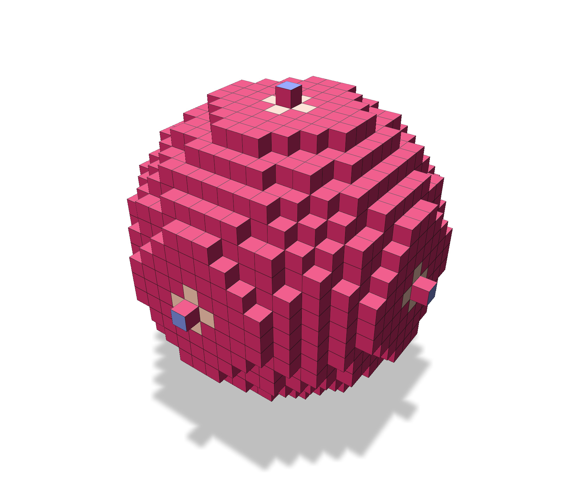
Table below shows in **yellow** places where the digitized boundary might not be a manifold. It show in **cyan** (and **yellow**) places where the projection might not be 1-1. It shows in **magenta** places where the digitized boundary is a 2-manifold and has a 1-1 projection onto the smooth shape boundary.
| cylinder $h=0.125$ | torus $h=0.125$ | torus $h=0.0625$ |
| -------- | -------- | -------- |
| 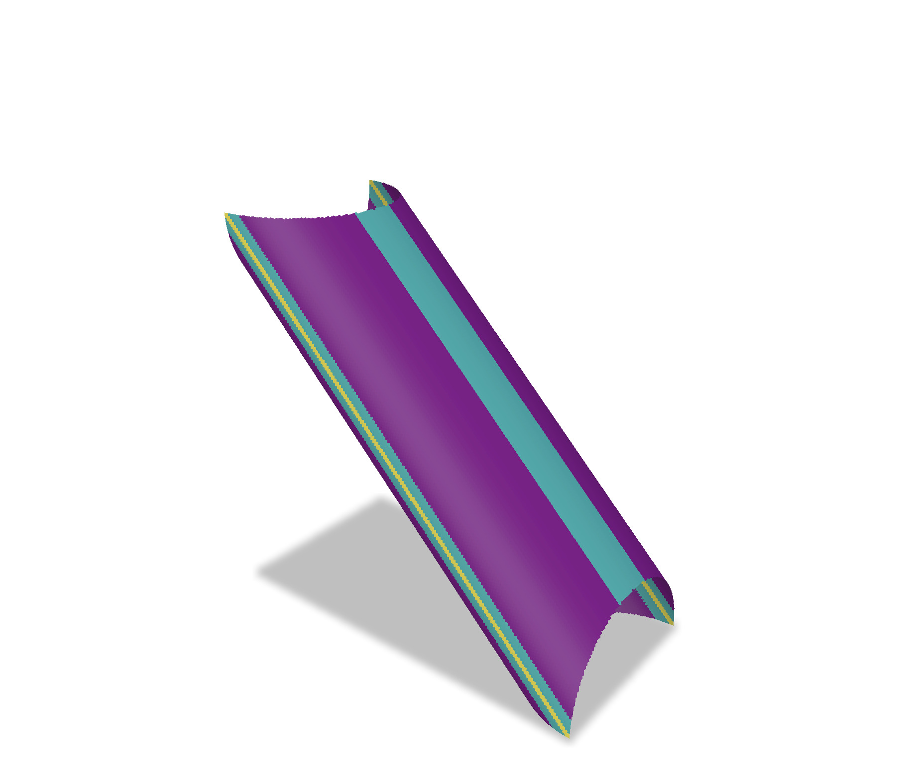 | 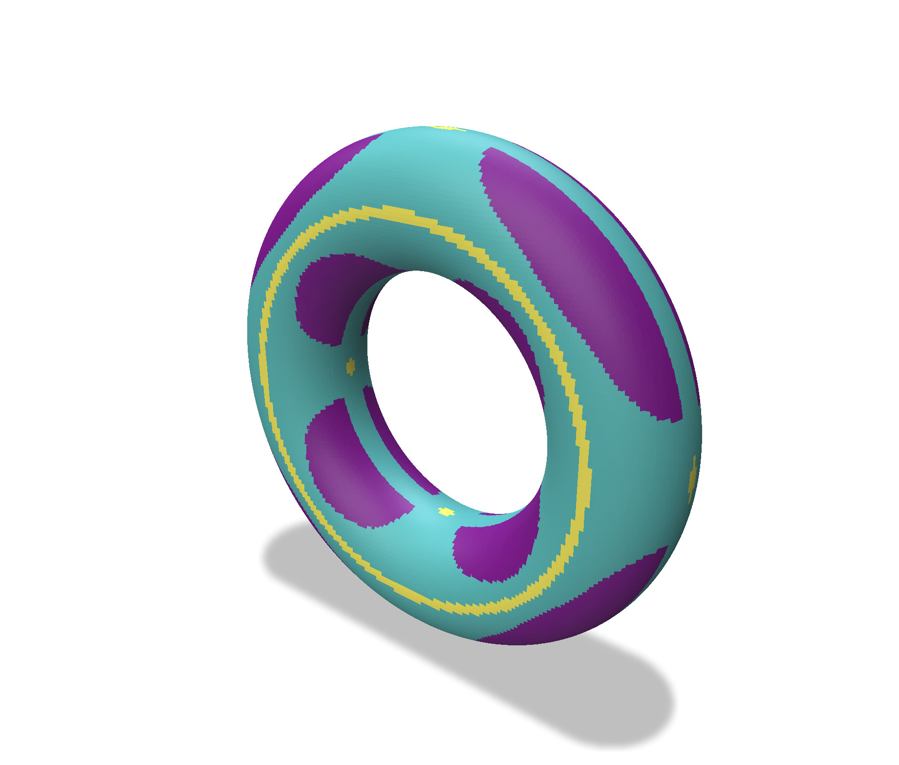 | 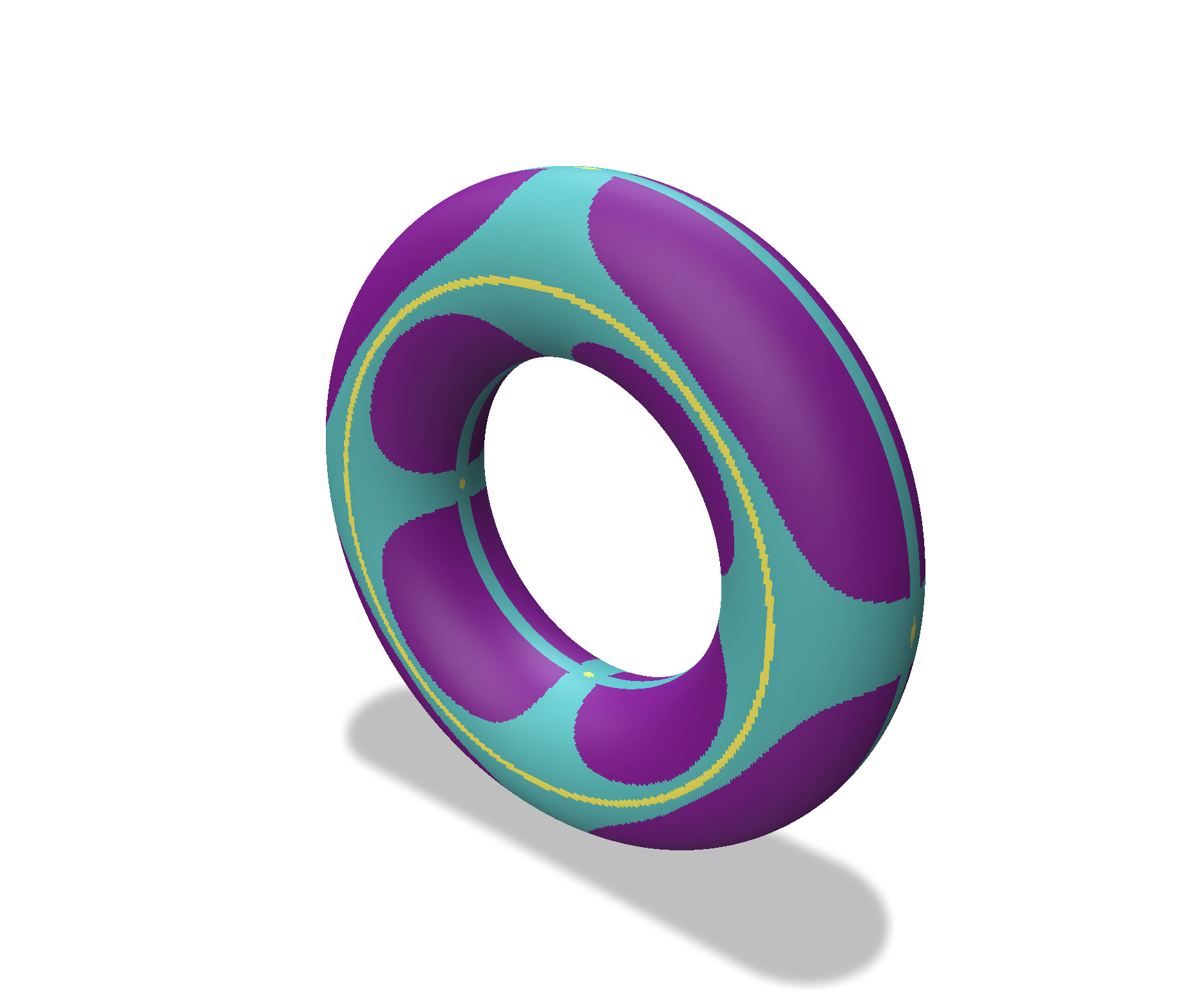 |
### Where the projection is 1-1 ?
Lemma 7 and Lemma 8 of [^5] together gives a sufficient condition to determine if your projection is locally 1-1. If the cosine of the angle between the normal $\mathbf{n}_i$ and any plane is greater than $2\sqrt{d}h/\rho$, then the projection $\pi$ onto $\partial \mathbf{X}$ is locally 1-1.
:::info
:::spoiler **Exercise**: computes the manifoldness and the 1-1 projection conditions
The manifoldness condition is easy to test by noticing that the smallest angle between the normal and an axis is $\cos^{-1}(\| \mathbf{n}_i \|_\infty)$. The 1-1 condition is easy to test by noticing that the sought cosine is the smallest component of $\mathbf{n}_i$ in absolute value.
:::
:::success
You may check that non-manifoldness implies not 1-1. As seen above, these are sufficient conditions, and are not tight at all in general. However they are enough --- and necessary --- to prove the multigrid convergence of the first area estimator.
:::
## References
[^1]: D. Coeurjolly, J.-O. Lachaud, and J. Levallois. Multigrid convergent principal curvature estimators in digital geometry. Computer Vision and Image Understanding, 129 :27 – 41, 2014.
[^2]: L. Cuel, J.-O. Lachaud, Q. Mérigot, and B. Thibert. Robust geometry estimation using the generalized voronoi covariance measure. SIAM Journal on Imaging Sciences, 8(2) :1293–1314, 2015.
[^3]: R. Klette and J. Žunic ́. Multigrid convergence of calculated features in image analysis. Journal of Mathematical Imaging and Vision, 13(3) :173–191, 2000.
[^4]: J.-O. Lachaud, D. Coeurjolly, and J. Levallois. Robust and convergent curvature and normal estimators with digital integral invariants. In L. Najman and P. Romon, editors,Modern Approaches to Discrete Curvature, volume 2184 of Lecture Notes in Mathema- tics, pages 293–348. Springer International Publishing, Cham, 2017.
[^5]: J.-O. Lachaud and B. Thibert. Properties of gauss digitized shapes and digital surface integration. Journal of Mathematical Imaging and Vision, 54(2) :162–180, 2016.
[^6]: J.-O. Lachaud and A. Vialard. Geometric measures on arbitrary dimensional digital surfaces. In G. Sanniti di Baja, S. Svensson, and I. Nyström, editors, Proc. Int. Conf. Discrete Geometry for Computer Imagery (DGCI’2003), Napoli, Italy, volume 2886 of LNCS, pages 434–443. Springer, 2003.