Uniform Sampling via Semi-Discrete Optimal Transport == > [name="Loïs Paulin"] [TOC] ## Warm-up: Downloading the code The skeleton of the code is available on [this Github Project](https://github.com/dcoeurjo/transport-optimal-gdrigrv-11-2020) (`semiDiscrete` folder). This code contains all you need compute and manipulate power diagrams (and to parse command line parameters for the `c++`code). You can download the archive from the Github interface (*"download zip"* menu), or *clone* the git repository. The project contains some `c++` and `python` codes. To compile the C++ tools, you would need [cmake](http://cmake.org) (>=3.14) to generate the project. For instance on linux/macOS: ``` bash git clone https://github.com/dcoeurjo/transport-optimal-gdrigrv-11-2020 cd transport-optimal-gdrigrv-11-2020 cd c++ mkdir build ; cd build cmake .. -DCMAKE_BUILD_TYPE=Release make ``` On Windows, use cmake to generate a Visual Studio project. The practical work described below can be done either in `c++` or `python`. ## Recap: Power Diagram and Semi-Discrete Optimal Transport Semi-Discrete Optimal Transport aims to transport a discrete distribution (a sum of diracs) onto a continuous distribution. Power diagrams are intrinsically linked to Semi-Discrete Optimal Transport: the map between each dirac and an area of equal measure minimizing Optimal Transport cost, called Optimal Transport Map, has been shown to be a power diagram with weights set such that each cell has a measure equal to that of its associated dirac[^power_transport]. In this tutorial we will see how to compute such weights and how this Optimal Tranport map can be used for point advection. ## Sampling via Optimal Transport The goal of sampling is to generate points (or dirac positions) distributed according to a continuous distribution on a given domain. Semi-Discrete Optimal Transport cost is commonly accepted as a good way to measure how well the samples match the target distribution. The smallest the cost the closer the discrete distribution is from the continuous one. The [Lloyd](https://en.wikipedia.org/wiki/Lloyd%27s_algorithm) algorithm is a classical sampling technique which iteratively advects an initial set of random samples to the centroids of their Voronoi cells. With an optimal transport view, this corresponds to iteratively computing for each Voronoi cell the dirac location which minimizes the transport cost to the cell points : the centroid of a cell $V$ can be viewed as the point minimizing the cost function $$ \mathbf{p} \mapsto \int_{\mathbf{x} \in V} \lVert \mathbf{x} - \mathbf{p} \rVert^2 \mathrm{d}\mu(\mathbf{x}), $$ which is a 2 Wasserstein distance. This algorithm however has no notion of capacity. Given $n$ points, we would like to ensure that the $n$ points are mapped to a $\frac{1}{n}$ portion of the target distribution. We have no guarantee here that the Voronoi cells of the sites correspond each to $\frac{1}{n}$ of the target measure. Our goal here is to generalize this algorithm into a two step iteration : 1. compute an optimal transport map between the set of $n$ samples considered as diracs with mass $\frac{1}{n}$ the mass of the target distribution and the target distribution. This is a semi-discrete optimal transport problem, which reduces to computing a set of weights for the sites, such that their power cells have the desired measure. 2. compute the optimal location for the dirac in the power cells to minimize the transport cost. These iterations are repeated until convergence to obtain a set of samples minimizing the transport cost to the target distribution. In this tutorial, we will implement this iteration using the the uniform distribution as a target distribution. ## The core We will aim at generating points minimizing optimal transport to the uniform distribution in a shape. 1. Get the `C++` / `python`. In Both cases, we provide elementary code to compute a power diagram restricted to an area. Get some time to understand how to use the underlying data structure. 2. With a uniform distribution, a cell measure is the area of its intersection with the shape. Write a function to compute a cell area. 3. We aim at finding weigths such that the difference between cell measure and point measure is minimized. If the cell measure is too small, the corresponding weight should increase. On the contrary, if the cell measure is too high, the weight should decrease. Write a gradient descent to minimize L1 norm of the difference (using the difference between target area and actual area as a gradient for each direction). 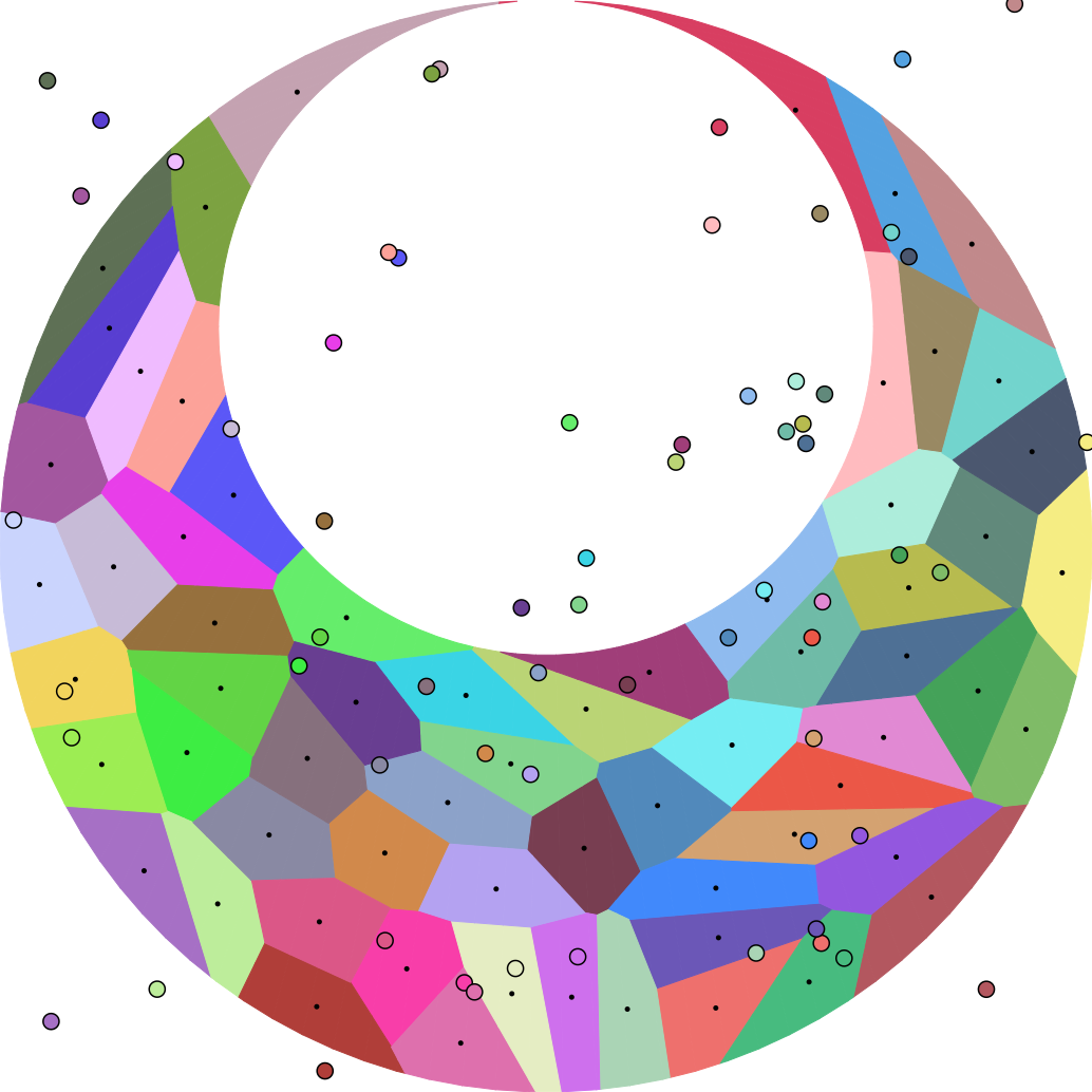With initialization from random points you should get something like this:  4. Once you have the Gradient descent minimization, output the final Wasserstein distance between a given set of samples and the uniform measure on the domain. You can observe the convergence by plotting the Wasserstein distance as a function of the number of iterations of the Gradient Descent. :::info Note that the energy being minized is convex and thus accepts more advanced solvers (e.g. multiscale Newton) for faster convergence[^quentin]. ::: 6. Now let's move the points to minimize the Wasserstein distance to uniform measure on the domain. Displace each point to the barycenter of its associated cell (Lloyd-like step). Again, iterate until convergence. :::info In the C++ version a given point cell might be splited in different mesh facets (one for each facet in your domain mesh) we give the function getCorrespondingPoint that takes a power diagram mesh and a facet index and returns which point is transported on it. ::: :::info In the code, we have added a tiny SVG exporter that allows you to visualize some vector graphic objects (poiints, polygons, ...). 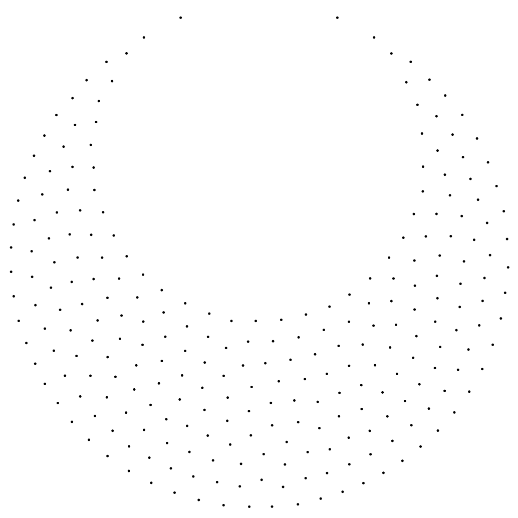::: You should obtain something like: {%youtube IzRkCb2ToBU%} Final points should look like this:  In higher dimension, computing the semi-discrete optimal transport using the Power diagram construction may be very expensive. Alternatively, we can consider a *sliced* approach to approximate efficiently the optimal transport cost[^spot]. 6. You can now play with your optimizer by setting differently shaped domains for your points (any triangulated mesh will do) or by changing target distribution and thus the way you compute the measure of a cell. Show us your best (or not) results. # References [^quentin]: A multiscale approach to optimal transport. Quentin Mérigot, Computer Graphics Forum 30 (5) 1583–1592, 2011 (also Proc SGP 2011) [^spot]: Sliced Optimal Transport Sampling, Loïs Paulin, Nicolas Bonneel, David Coeurjolly, Jean-Claude Iehl, Antoine Webanck, Mathieu Desbrun, Victor Ostromoukhov, ACM Transactions on Graphics (Proceedings of SIGGRAPH), July 2020 [^power_transport]: Minkowski-Type Theorems and Least-Squares Clustering, Franz Aurenhammer, Friedrich Hoffman, Boris Aronov, Algorithmica 20, January 1998