[CGDI] Bilateral Filtering (and sliced optimal transport again) == In this practical, we will implement image denoising using a bilateral filter before going back to the sliced optimal transport problem (cf practical #1). | | | | -------- | -------- | | 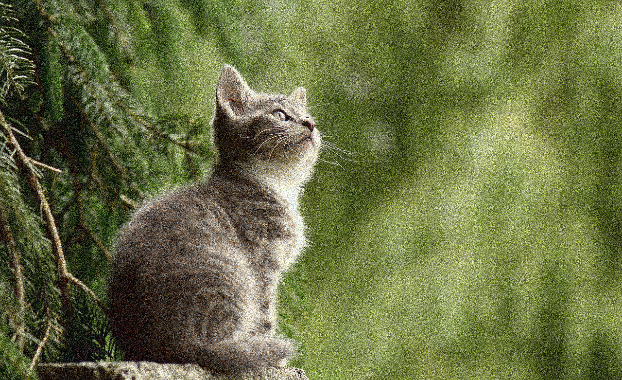 | 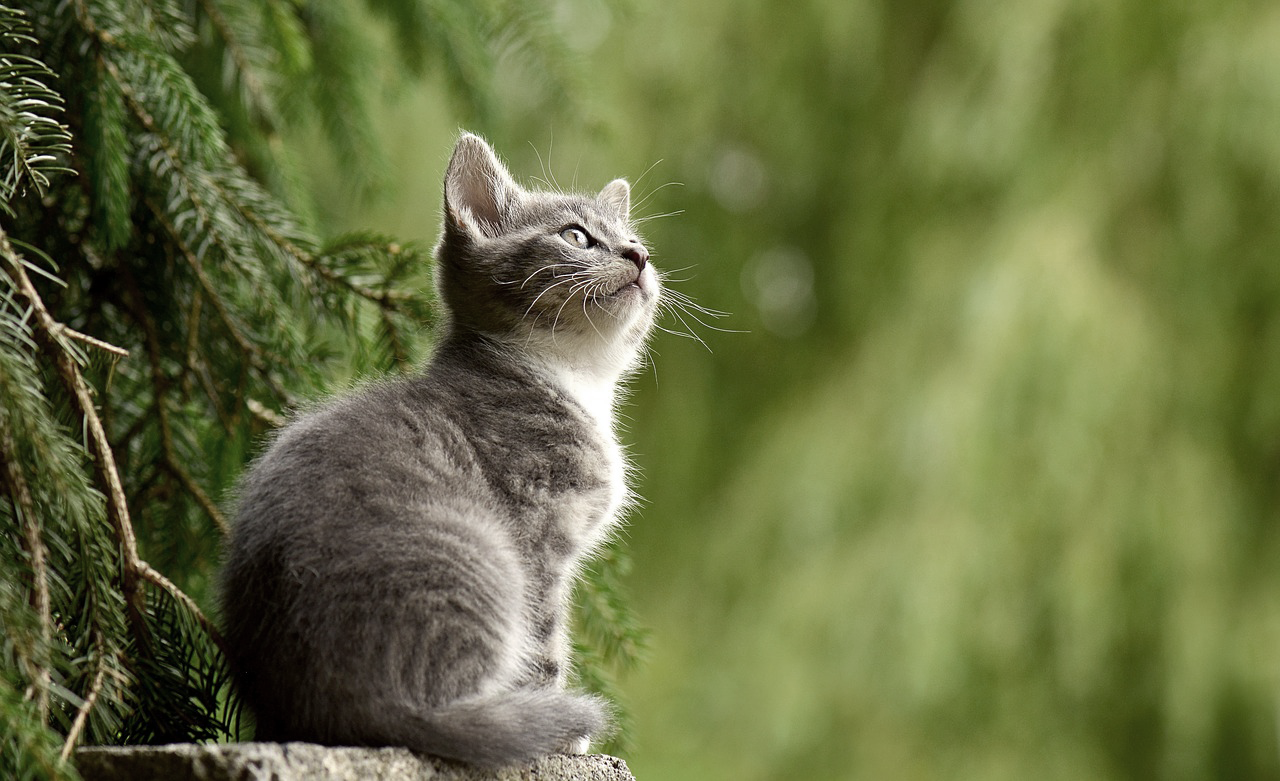 | # Warmup 1: Gaussian convolution 1. Implement a Gaussian filter that can be parametrized by the kernel standard deviation $\sigma$. Remember, the Gaussian filter being separable, only a 1D filter is needed here (check your lecture notes) 2. Observe the filtering results on the cat while increasing the $\sigma$. How does this affect the computational cost? 3. Can you list some boundary strategies to deal with the image border? 4. There are many high performance implementations. Have a quick look to the [Recursive Gaussian Filters](https://hal.inria.fr/inria-00074778/document) approach (e.g. Eq(35)). What is the main interest of this kind of technique? 5. As the convolution corresponds to a pointwise product in Fourier domain, how can we use this spectral approach for fast Gaussian filtering? # Warmup 2: Median filter 1. The median filter replace the pixel value by the median of the pixel values in the Kernel. Implement such filter (`std::sort` is your friend). 2. How does this filter compare to the Gaussian filter (efficiency, complexity...)? # Bilateral Filtering The bilateral filter is a very popular non-linear, edge preserving smoothing filter. The main idea is to filter the pixel values in both the spatial and the range domains.  More formally, a smoothed image $I^*$ is given by: $$ I^*(x) = \frac{1}{W} \sum_{y \in \Omega_x} I(y)f(|I(y)-I(x)|)g(\|y-x\|), $$ with * $W= \sum_{y\in \Omega_x}{f(|I(y)-I(x)|)g(\|y-x\|)}$ (the normalization factor); * $\Omega_x$ is a window around $x$; * $f$ and $g$ are decreasing functions $[0,+\infty]\rightarrow\mathbb{R}^+$.  In the context of this practical, both $f$ and $g$ will be (halves of) Gaussian kernels. 1. Is the bilateral filter separable? 2. What is the computational cost of a separable implementation of the Gaussian filtering (with fixed width $w$ or instance)? What is the computational cost of a naive implementation of the bilateral filter? 3. Provide a direct implementation of the bilateral filter and use it on the noisy images provided in the github project. 4. A fast implementation of the bilateral filter exists[^Chen], please have a look to the paper. The basic idea is to transform the anisotropic bilateral filter into a simple Gaussian filtering in higher dimensions. Using the separable Gaussian filter you may already have, implement such an approach and compare its performances with respect to the direct implementation. # Sliced Optimal Transport Now let's go back to the [SOT project](https://codimd.math.cnrs.fr/s/s_rh7X9wF) and complete it. The bilateral filter will be used as a regularizer of the transport map (cf question 8). If you want a simple python code to compute the color histograms (per channel) of an image, here you have a [python code](https://raw.githubusercontent.com/dcoeurjo/transport-optimal-gdrigrv-11-2020/main/misc/computeHistogram.py). # References [^Chen]: Chen, Jiawen, Sylvain Paris, and Fredo Durand. "Real-time edge-aware image processing with the bilateral grid." ACM Transactions on Graphics (TOG). Vol. 26. No. 3. ACM, 2007. [PDF](https://citeseerx.ist.psu.edu/document?repid=rep1&type=pdf&doi=2760e681e9962fe56f4849aff25aecbecbe89ec6)