Practical: Homotopic Thinning
==
> David Coeurjolly
The objective of this practical is to implement an homotopic thinning algorithm of a 3d binary object using [DGtal](https://dgtal.org).
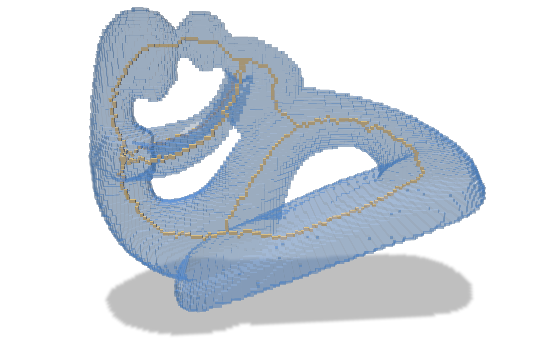
| Input | Step 1. | .. | Step k | .. | Final |
| ----------------------|----------|---------------------------------------------------- | -------- | -------- |-----------|
| 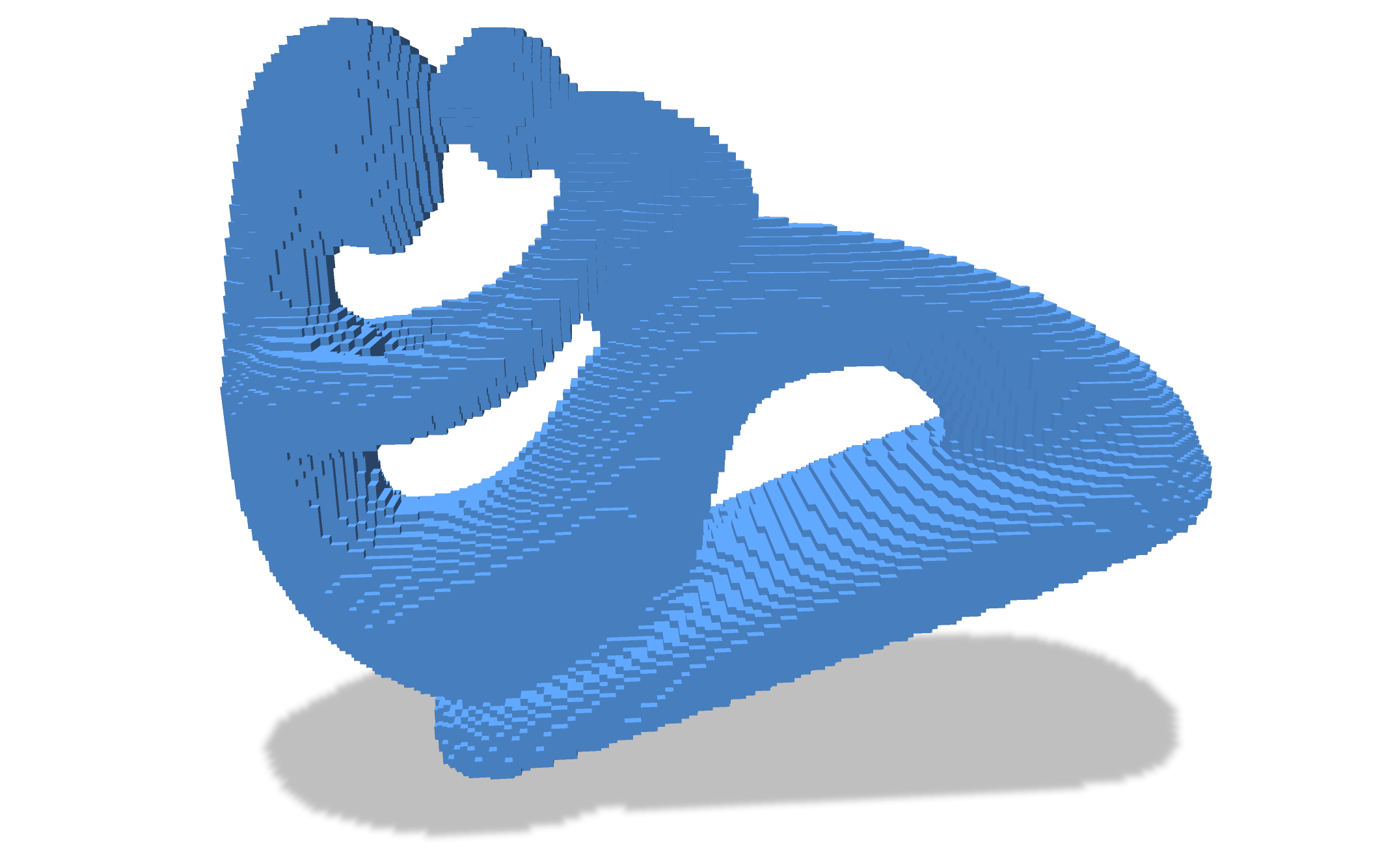 | 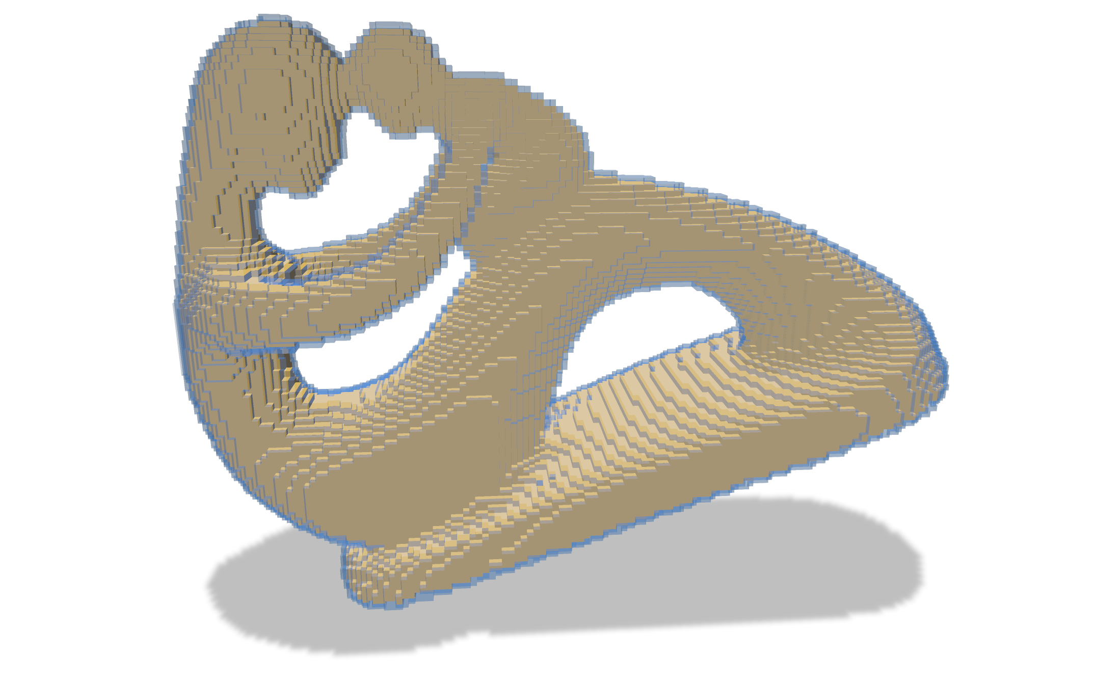| ... | 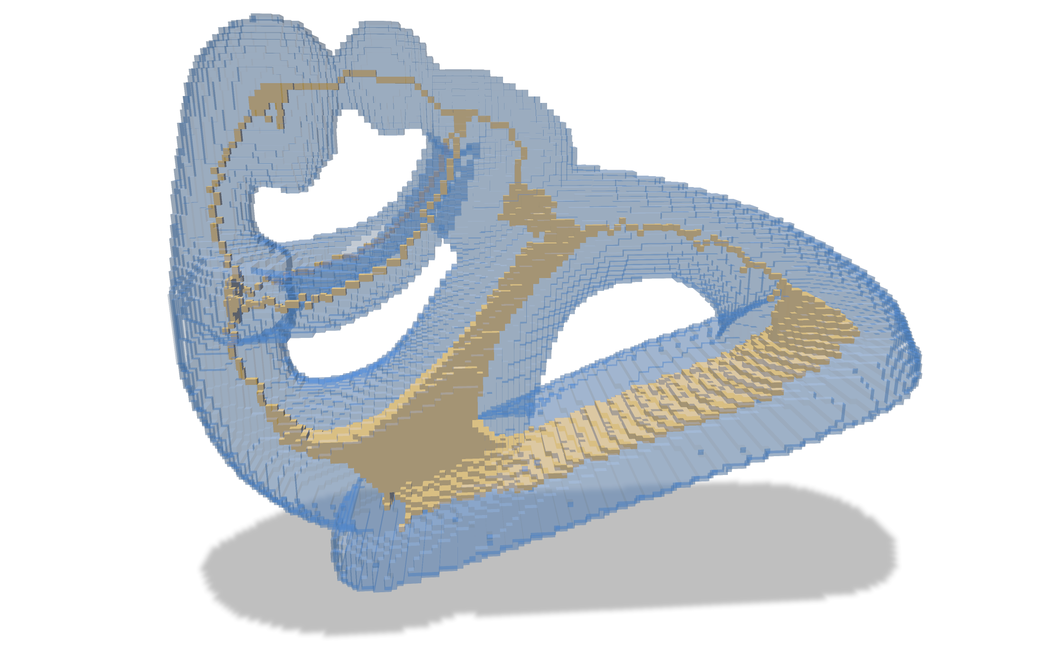| ... |
[TOC]
# Getting Started
In the DGtal-DGMM repository, have a look to the `homotopic-thinning.cpp` file. It should compile as is and if you provide an input Vol file in the command line
```
./homotopic-thinning -i fertility-128.vol
```
:::danger
:::spoiler Performances
When you code is up and running on small volumetric files, make sure to compile the project in cmake `Release` mode to get best performances (internal asserts will be disabled).
:::
You should see a polyscope window with two surface meshes: the input digital object primal surface and the thinned object primal surface.
:::success
:::spoiler Primal surface?
The primal surface of a digital object corresponds to an embedding of the [digital surface](https://dgtal-team.github.io/doc-nightly/moduleDigitalSurfaces.html) (boundary of the union of the voxels) in the [Khalimsky grid](https://dgtal-team.github.io/doc-nightly/moduleCellularTopology.html), to the Euclidean space. I.e. 2-cells (cells of dimension 2 of the Khalimsky complex) corresponding to the boundary between interior and exterior voxels are embedded as unit squares.
:::
# The algorithm
## Preliminaries
The main part of the documentation for this practical is the one related to [digital topology and objects](https://dgtal-team.github.io/doc-nightly/moduleDigitalTopology.html).
In terms of data structures, [DGtal](https://dgta.org) makes the distinction between:
* [Domains](https://dgtal-team.github.io/doc-nightly/moduleSpacePointVectorDomain.html): digital domain. For instance, types `Z2i::Domain` and `Z3i::Domain` correspond to hyper rectangular domains defined by two points (lower and upper-bound) in dimensions 2 and 3.
* [Digital sets](https://dgtal-team.github.io/doc-nightly/moduleDigitalSets.html): containers for point sets in a given domain. For example, once constructed, points can be inserted, removed. E.g.
:::success
:::spoiler Digital Sets containers and Concepts
Internally, many data structures can be used to implement a digital set container (`std::set, std::unorderd_set, std::vector, user-specified data structure...`). Each **model** of digital sets must satisfy the concept of Digtal Set (must have the same API, same preconditions...). In DGtal, we use boost concepts for that. Have a look to the [CDigitalSet](https://dgtal-team.github.io/doc-nightly/structDGtal_1_1concepts_1_1CDigitalSet.html) concept file.
:::
``` c++
Z3i::Point a(0,0,0);
Z3i::Point b(64,64,64);
Z3i::Domain domain( a,b );
Z3i::DigtalSet aSet( domain );
Z3i::Point p(42,42,42);
aSet.insert( p );
aSet.erase( p );
...
```
* [Digital Objects](https://dgtal-team.github.io/doc-nightly/moduleDigitalTopology.html): a digital set equipped with a topological structure (Adjacency relation). In 2d, classical [DigitalTopology](https://dgtal-team.github.io/doc-nightly/classDGtal_1_1DigitalTopology.html) models are `Z2i::DT4_8` and `Z2i::DT_8_4`. In 3d, we have the shortcuts `Z3i::DT6_26`, `Z3i::DT26_6`, `Z3i::DT6_18` and `Z3i::DT18_6` that define proper Jordan pairs of adjacency relationships. Note that if you have your own definitions for the adjacency at the object and its background, you can instantiate a Digital Object on it. On [Object](https://dgtal-team.github.io/doc-nightly/classDGtal_1_1Object.html) instances, you can compute several topological quantities such as the border of an object or [the simplicity of a point](https://dgtal-team.github.io/doc-nightly/moduleDigitalTopology.html#dgtal_topology_sec3_5).
:::info
For the `Z3i::DT6_26` topology, the associated DigitalObject can be simply instantiating using the `Z3i::Object6_26` type.
:::
E.g.:
``` c++
... //continuing with the previous code snippet
Z3i::Object6_26 anObject( aSet );
bool is_p_simple = anObject.isSimple( p );
//should return false here.
...
```
:::success
:::spoiler Simple points?
Roughly speaking, for a given digital object, a point is simple if removing it does not change some topological invariants of the object and its complement (e.g. number of holes, number of connected components, number of tunnels...). See [^1] for a more formal definition.
:::
## Homotopic Thinning
The object is to implement a layered homotopic thinning algorithm. For a 3d digital object, the algorithm can be sketched as follows:
* We detect and store all points that are simple
* Then, for all simple poins, we remove them one by one (when removing a point, we must check that the point is still simple).
* We repeat until no more simple points exist.
The fixed point of the algorithm is thus a 1d curvilinear skeleton with is homotopic to the input one.

# Let's go
1. Have a look to the code skeleton `practical-homotopic-thinning/homotopic-thinning.cpp`. You will have everything to load a Vol file (in the [data](https://github.com/DGtal-team/DGtal-Tutorials-DGMM2022/tree/main/data) folder or [VolGallery](https://github.com/dcoeurjo/VolGallery)), construct the digital object and visualize the boundary of an binary image using [polyscope](https://polyscope.run).
2. Implement the main method `oneStep()` that performs one step of the above-described algorithm.
3. Change the adjacency pairs of the digital object and compare the results.
:::info Tips
**Tips**:
* You would have to maintain two structures: the digital object that is peeled, and the binary image ($\mathbb{Z}^3\rightarrow \{0,1\}$) that is used for the visualization.
* In polyscope, the `Options` button on a mesh structure opens up a panel in which you can play with the transparency of the surface.
* For efficiency purposes, the simplicity test is performed using a precomputed lookup table, available in 2d or 3d. In higher dimensions, we fall back on the explicit computation of connected components as described in [^1].
:::
# Going further
The naive algorithms can be enhanced in many ways:
* You can add anchor points: for a given predicate returning true if a point is an anchor point, update the code to remove simple points that do not satisfy the predicate (and find an interesting predicate;))
* When processing the simple points, a priority queue can be considered based on the distance transformation of the object. Use the [separable distance transformation](https://dgtal-team.github.io/doc-nightly/moduleVolumetric.html) algorithm to order the points.
# References
[^1]: Gilles Bertrand and Grégoire Malandain. A new characterization of three-dimensional simple points. Pattern Recognition Letters, 15(2):169–175, February 1994.