---
title: IPCV Practical - Homotopic Thinning
---
# IPCV Practical - Homotopic Thinning
> Course [Digital geometry processing](https://codimd.math.cnrs.fr/s/dc2zU_Cui) (<a href="ipcv.eu"> Master IPCV </a>)
> [name=David Coeurjolly][time=Nov 2022][color=#fe1122]
> [name=Jacques-Olivier Lachaud][time=Dec 2025][color=#907bf7]
###### tags: `lecture` `digital geometry` `geometry processing` `DGtal` `3d` `digital topology`
The objective of this practical is to implement an homotopic thinning algorithm of a 3d binary object using [DGtal](https://dgtal.org).
| Input | | Step 1 | ... |
| ------------------------------------------------------------------------------------ | ------- | ------------------------------------------------------------------------------------ | --- |
| 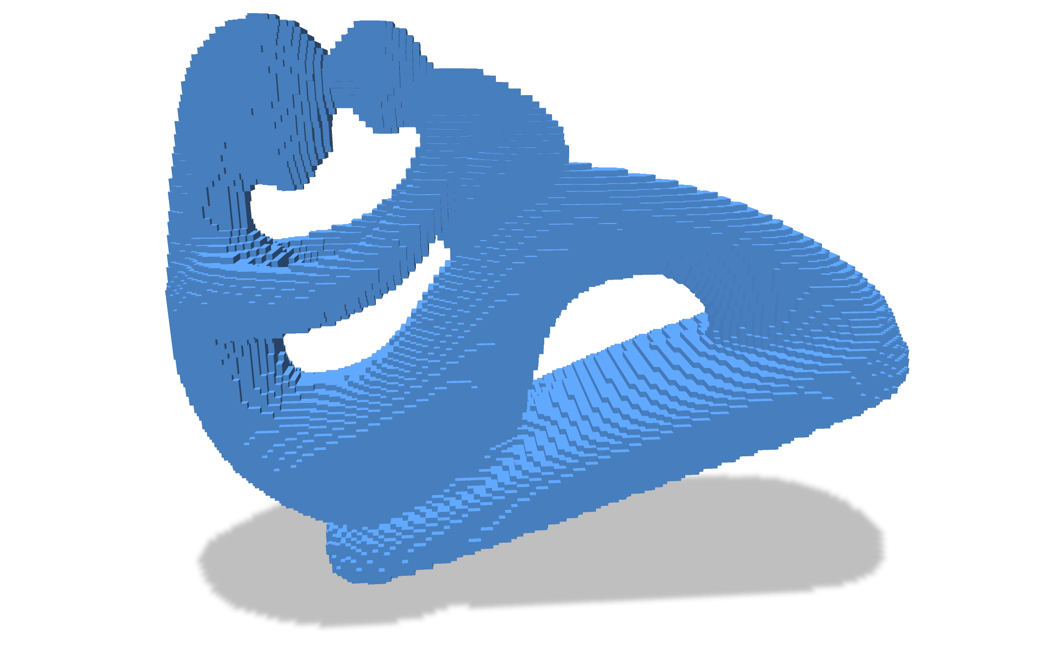 | | 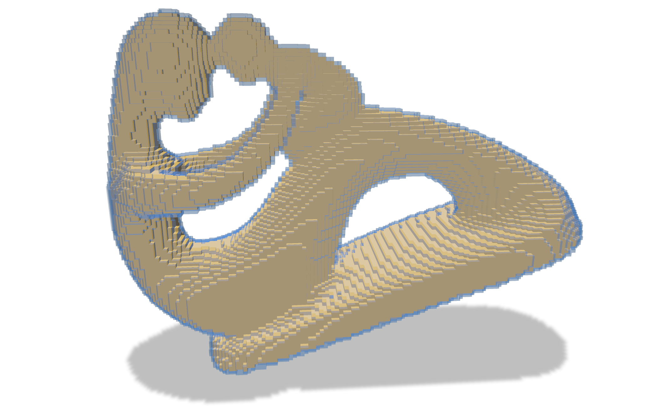 | |
| **Step $k$** | **...** | **Final** | |
| 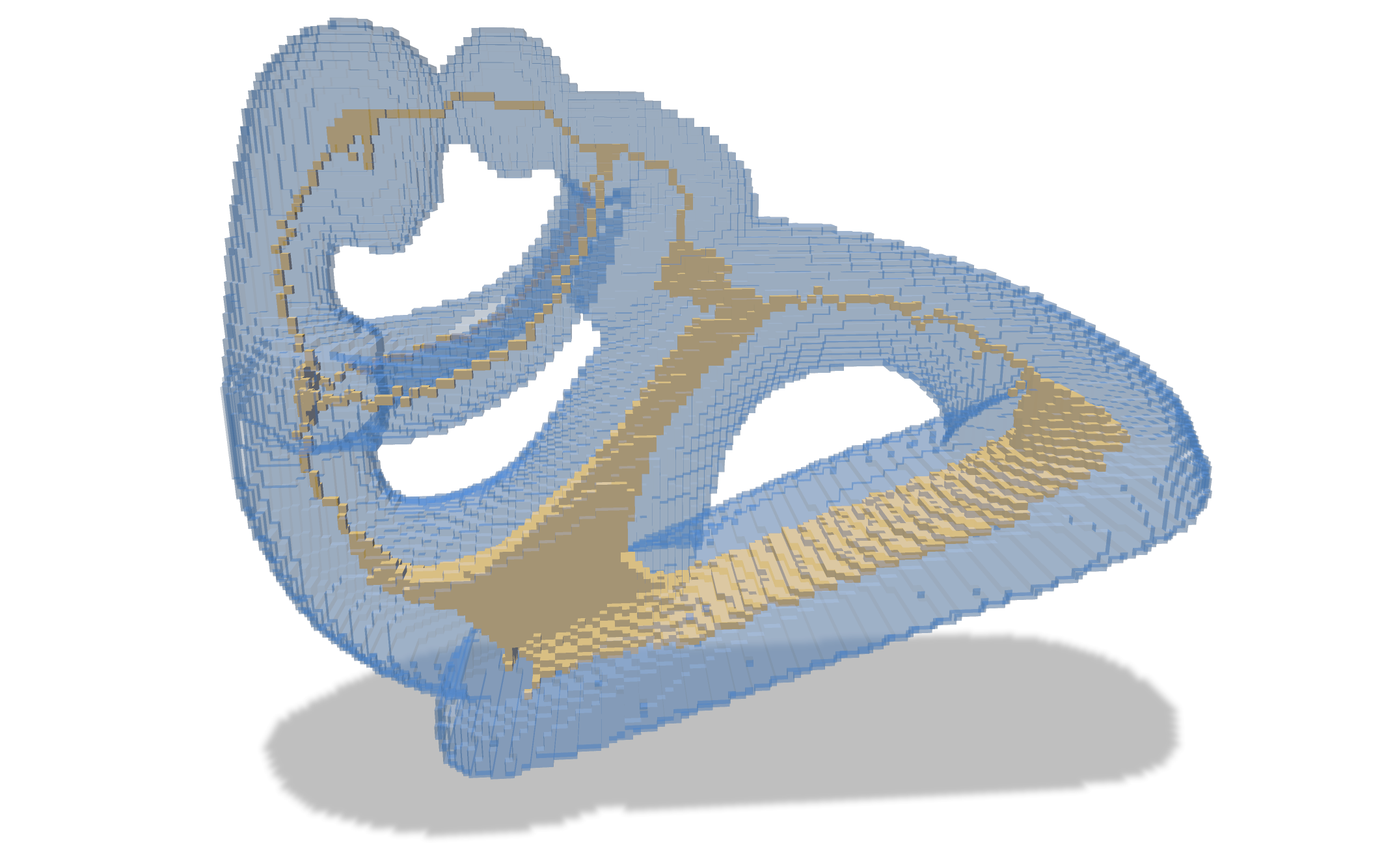 | | 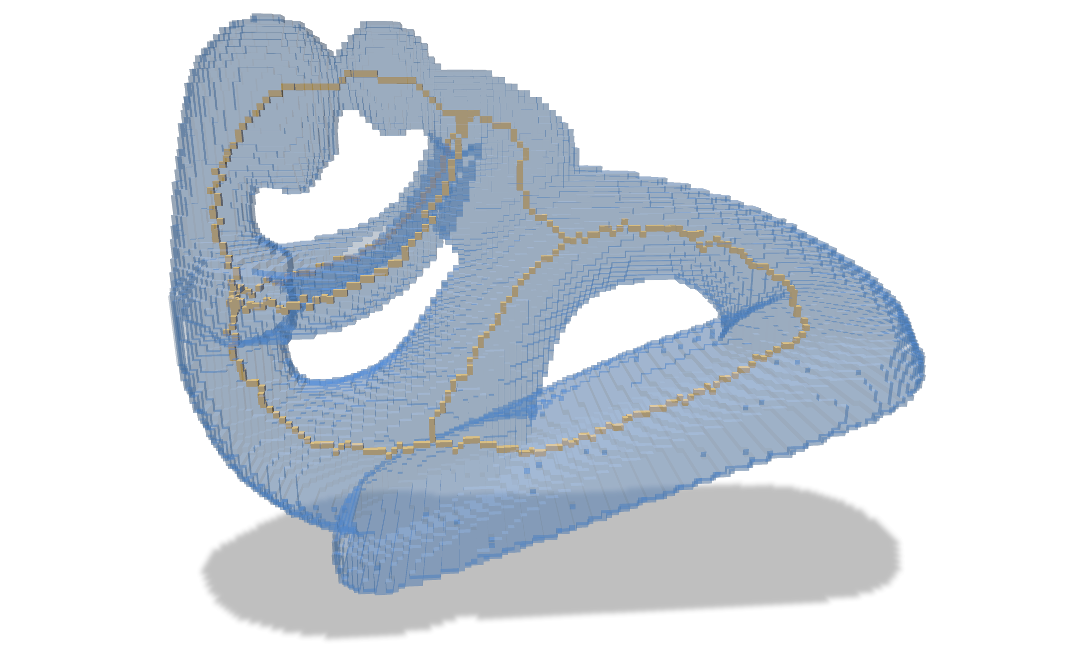 | |
[TOC]
## Getting Started
In the DGtal-DGMM repository, have a look to the `homotopic-thinning.cpp` file. It should compile as is and if you provide an input Vol file in the command line
```
./homotopic-thinning -i ../data/fertility-128.vol
```
:::danger
:::spoiler Performances
When you code is up and running on small volumetric files, make sure to compile the project in cmake `Release` mode to get best performances (internal asserts will be disabled).
:::
You should see a polyscope window with two surface meshes: the input digital object primal surface and the thinned object primal surface.
:::success
:::spoiler Primal surface?
The primal surface of a digital object corresponds to an embedding of the [digital surface](https://dgtal-team.github.io/doc-nightly/moduleDigitalSurfaces.html) (boundary of the union of the voxels) in the [Khalimsky grid](https://dgtal-team.github.io/doc-nightly/moduleCellularTopology.html), to the Euclidean space. I.e. 2-cells (cells of dimension 2 of the Khalimsky complex) corresponding to the boundary between interior and exterior voxels are embedded as unit squares.
:::
## The algorithm
### Preliminaries
The main part of the documentation for this practical is the one related to [digital topology and objects](https://dgtal-team.github.io/doc-nightly/moduleDigitalTopology.html).
In terms of data structures, [DGtal](https://dgta.org) makes the distinction between:
* [Domains](https://dgtal-team.github.io/doc-nightly/moduleSpacePointVectorDomain.html): digital domain. For instance, types `Z2i::Domain` and `Z3i::Domain` correspond to hyper rectangular domains defined by two points (lower and upper-bound) in dimensions 2 and 3.
* [Digital sets](https://dgtal-team.github.io/doc-nightly/moduleDigitalSets.html): containers for point sets in a given domain. For example, once constructed, points can be inserted, removed. E.g.
:::success
:::spoiler Digital Sets containers and Concepts
Internally, many data structures can be used to implement a digital set container (`std::set, std::unorderd_set, std::vector, user-specified data structure...`). Each **model** of digital sets must satisfy the concept of Digtal Set (must have the same API, same preconditions...). In DGtal, we use boost concepts for that. Have a look to the [CDigitalSet](https://dgtal-team.github.io/doc-nightly/structDGtal_1_1concepts_1_1CDigitalSet.html) concept file.
:::
``` c++
Z3i::Point a(0,0,0);
Z3i::Point b(64,64,64);
Z3i::Domain domain( a,b );
Z3i::DigtalSet aSet( domain );
Z3i::Point p(42,42,42);
aSet.insert( p );
aSet.erase( p );
...
```
* [Digital Objects](https://dgtal-team.github.io/doc-nightly/moduleDigitalTopology.html): a digital set equipped with a topological structure (Adjacency relation). In 2d, classical [DigitalTopology](https://dgtal-team.github.io/doc-nightly/classDGtal_1_1DigitalTopology.html) models are `Z2i::DT4_8` and `Z2i::DT_8_4`. In 3d, we have the shortcuts `Z3i::DT6_26`, `Z3i::DT26_6`, `Z3i::DT6_18` and `Z3i::DT18_6` that define proper Jordan pairs of adjacency relationships. Note that if you have your own definitions for the adjacency at the object and its background, you can instantiate a Digital Object on it. On [Object](https://dgtal-team.github.io/doc-nightly/classDGtal_1_1Object.html) instances, you can compute several topological quantities such as the border of an object or [the simplicity of a point](https://dgtal-team.github.io/doc-nightly/moduleDigitalTopology.html#dgtal_topology_sec3_5).
:::info
For the `Z3i::DT6_26` topology, the associated DigitalObject can be simply instantiating using the `Z3i::Object6_26` type.
:::
E.g.:
``` c++
... //continuing with the previous code snippet
Z3i::Object6_26 anObject( aSet );
bool is_p_simple = anObject.isSimple( p );
//should return false here.
...
```
:::success
:::spoiler Simple points?
Roughly speaking, for a given digital object, a point is simple if removing it does not change some topological invariants of the object and its complement (e.g. number of holes, number of connected components, number of tunnels...). See [^1] for a more formal definition.
:::
### Homotopic Thinning
The object is to implement a layered homotopic thinning algorithm. For a 3d digital object, the algorithm can be sketched as follows:
* We detect and store all points that are simple
* Then, for all simple points, we remove them one by one.
:warning: when removing a point, we must check again that the point is still simple, because the neighborhood may have changed in-between.
* We repeat until no more simple points exist.
The fixed point of the algorithm is thus a 1d curvilinear skeleton which is homotopic to the input one.

## Let's go
1. Have a look to the code skeleton `practical-homotopic-thinning/homotopic-thinning.cpp`. You will have everything to load a Vol file (in the [data](https://github.com/DGtal-team/DGtal-Tutorials-DGMM2022/tree/main/data) folder or [VolGallery](https://github.com/dcoeurjo/VolGallery)), construct the digital object and visualize the boundary of an binary image using [polyscope](https://polyscope.run).
2. To better understand the construction of the digital object and the extraction of its boundary, you may have a look at the [Shortcuts module](https://www.dgtal.org/doc/stable/moduleShortcuts.html)
3. Implement the main method `oneStep()` that performs one step of the above-described algorithm.
4. Change the adjacency pairs of the digital object and compare the results. Update the polyscope GUI so that we can choose between (26,6) and (6,26)
:::info Tips
**Tips**:
* You would have to maintain two structures: the digital object that is peeled, and the binary image ($\mathbb{Z}^3\rightarrow \{0,1\}$) that is used for the visualization.
* In polyscope, the `Options` button on a mesh structure opens up a panel in which you can play with the transparency of the surface.
* For efficiency purposes, the simplicity test is performed using a precomputed lookup table, available in 2d or 3d. In higher dimensions, we fall back on the explicit computation of connected components as described in [^1].
:::
## Going further
The naive algorithms can be enhanced in many ways:
### 1. Add anchor points
You can add anchor points: for a given predicate returning true if a point is an anchor point, update the code to remove simple points that do not satisfy the predicate (and find an interesting predicate :wink:).
As example of anchor point, one could chose points that have only 1 neighbor in their 26 neighborhood (a kind of end point).
### 2. Process simple points in order following their depth
When processing the simple points, a priority queue can be considered based on the distance transformation of the object. Use the [separable distance transformation](https://dgtal-team.github.io/doc-nightly/moduleVolumetric.html) algorithm to order the points.
Instead of peeling layer by layer, you process points one at a time according to its distance to the boundary (i.e. its depth). If it is simple, the point is deleted, otherwise it is kept.
The resulting skeleton is better centered in the original shape.
### 3. Using more elaborate thinning algorithms
There are more subtle ways of thinning digital objects. Generally, you not only wish to keep the global topology, but also some local topologic or geometric characteristics. For instance, you wish to preserve the curve parts, or some surfacic parts of the shape, or keep some anchor points.
**Asymmetric thinning based on critical kernels** is a way to thin an object while keeping its 1d or 2d parts [^2][^3][^4]. You may have a look at its [description in DGtal documentation]((https://dgtal-team.github.io/doc-nightly/moduleVoxelComplex.html), and also check the code of the tool [criticalKernelsThinning3D](https://dgtal-team.github.io/doctools-nightly/criticalKernelsThinning3D_8cpp_source.html) in [DGtalTools](https://dgtal-team.github.io/doctools-nightly/group__volumetrictools.html).
We compare below the result of different thinning algorithms on input image `PA05-lbl.vol`, a segmented image of a human artery pulmonary system (non segmented image is `PA05-img.vol`).
* 25 thinnings: just applying $25 \times$ the `oneStep` thinning function, which removes one layer of simple points each time.
* isthmus thinning (p=10): preserves isthmus while thinning, with a persistence of 10. It tends to build surfacic skeleton, but it is in general too noisy (for small persistence). A persistence of 10 keeps only deep enough surfacic skeleton (2-isthmus) points.
* 1-isthmus thinning (p=1): preserves 1-isthmus while thinning, with a persistence of 1. It builds curvilinear skeleton. **This is clearly the most interesting method here**, since it detects the whole vascular system of the lungs. It would be easy to measure its length here, just by counting the points.
| Input | Input+25 thinnings | 25 thinnings |
| ---------------------------------------------------------------------------------------------- | ---------------------------------------------------------------------------------------------- | ----------------------------------------------------------------------------------------------- |
| 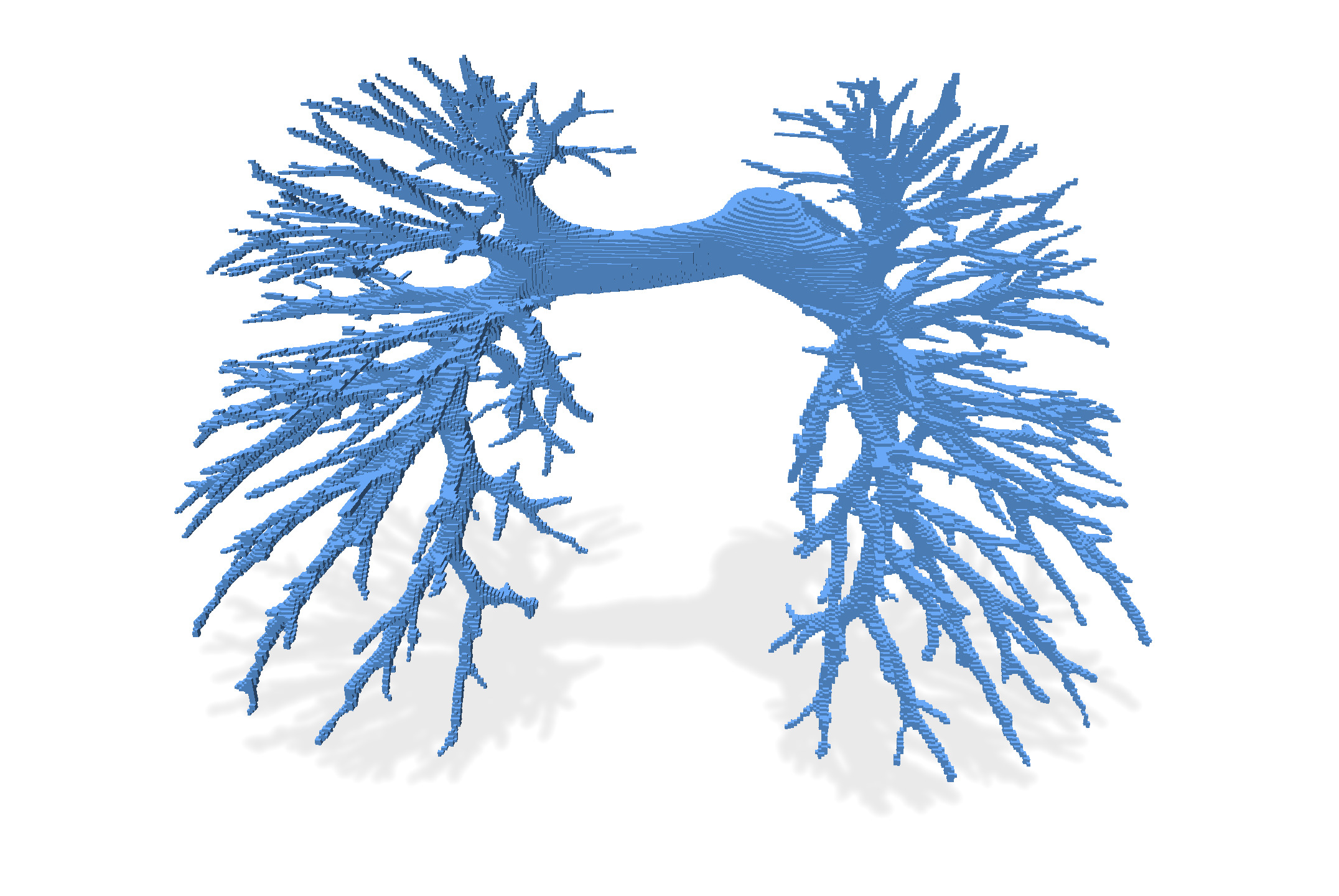 |  | 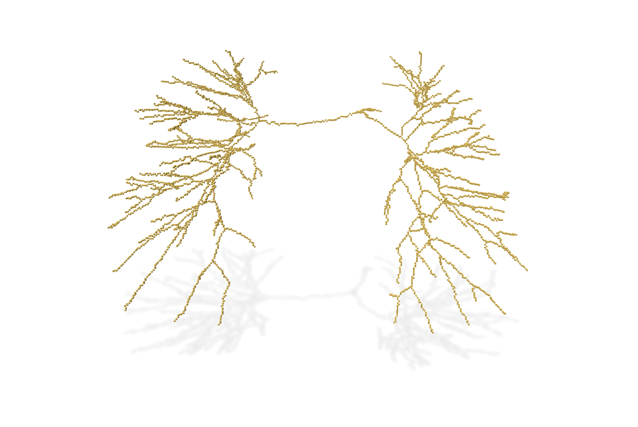 |
| Input | Input+ isthmus thinning $(p=10)$ | isthmus thinning $(p=10)$ |
|  | 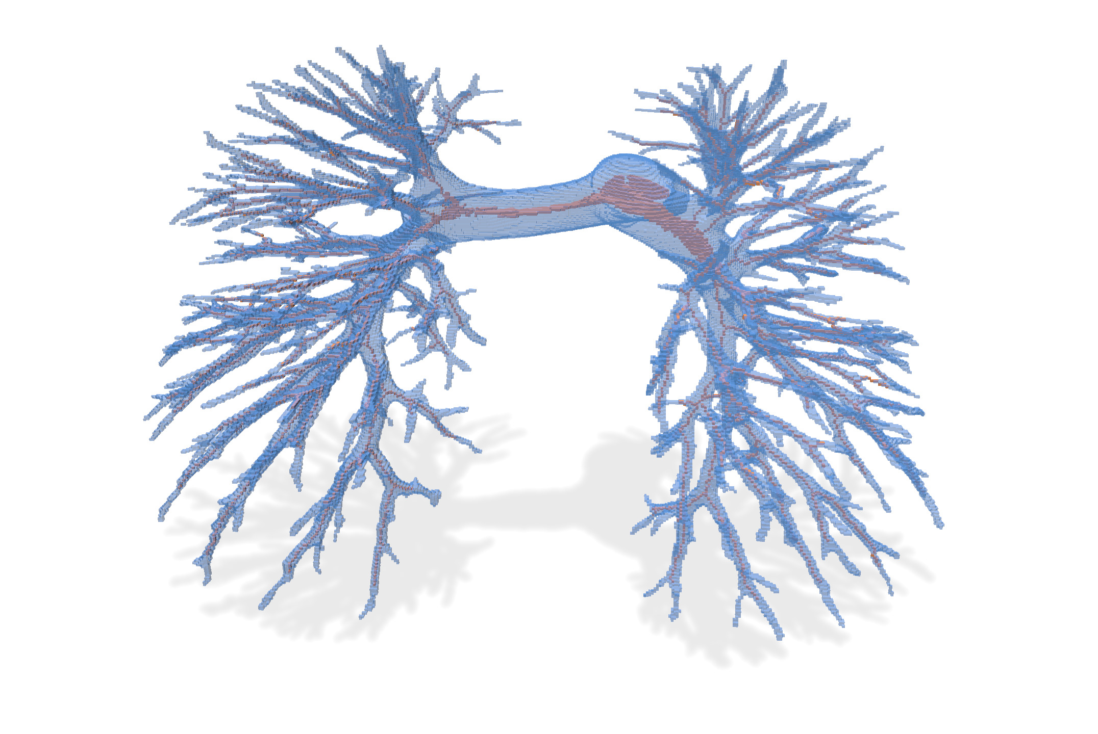 | 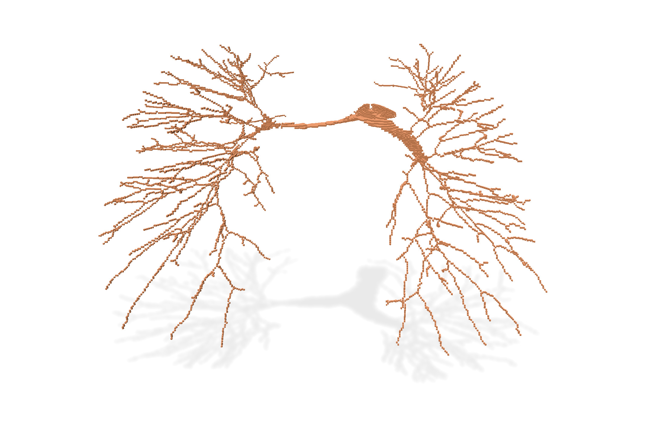 |
| Input | Input+ 1-isthmus thinning $(p=1)$ | 1-isthmus thinning $(p=1)$ |
|  | 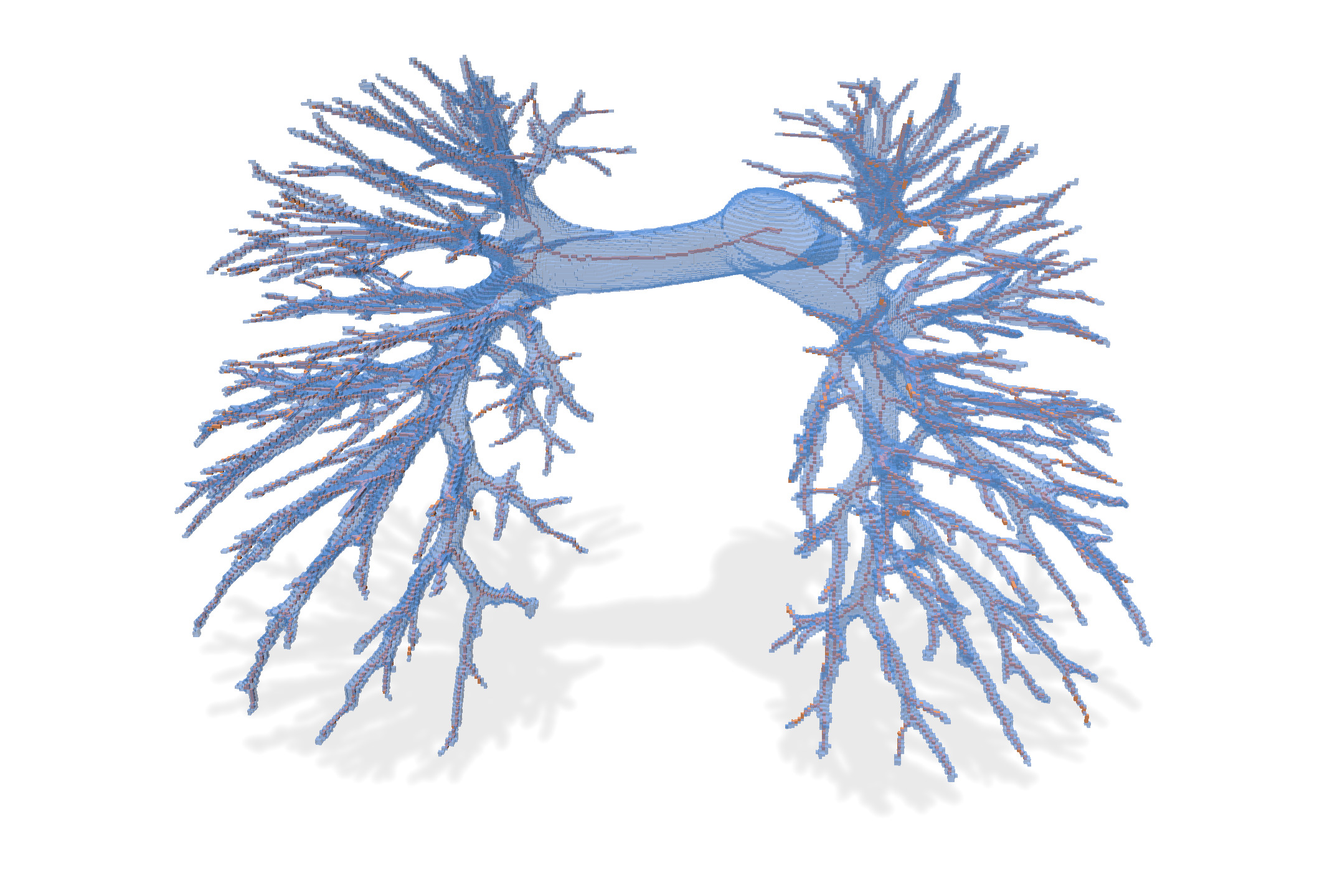 | 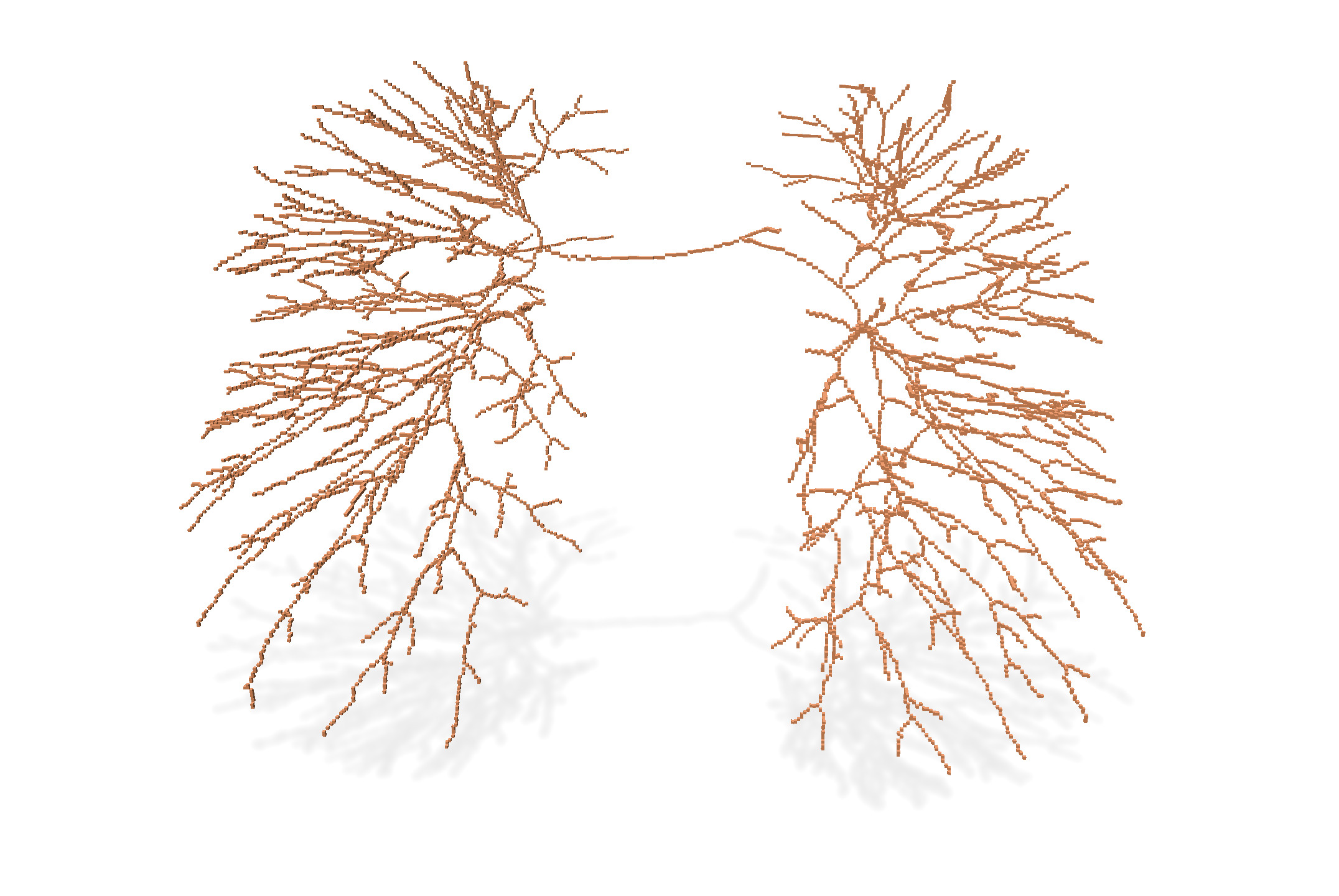 |
## References
[^1]: Gilles Bertrand and Grégoire Malandain. A new characterization of three-dimensional simple points. Pattern Recognition Letters, 15(2):169–175, February 1994.
[^2]: Michel Couprie, Gilles Bertrand. Asymmetric parallel 3D thinning scheme and algorithms based on isthmuses: https://hal.archives-ouvertes.fr/hal-01217974/document
[^3]: Gilles Bertrand, Michel Couprie. Powerful Parallel and Symmetric 3D Thinning Schemes Based on Critical Kernels: https://hal.archives-ouvertes.fr/hal-00828450/
[^4]: Michel Couprie, Gilles Bertrand. A 3D Sequential Thinning Scheme Based on Critical Kernels: https://hal.archives-ouvertes.fr/hal-01217952/file/Critical3Dseq.pdf