[CGDI] Monte Carlo Geometry Processing === > [name="David Coeurjolly"] ENS [CGDI](https://perso.liris.cnrs.fr/vincent.nivoliers/cgdi/) [TOC] --- The objective of this practical is to use path tracing and Monte Carlo sampling concepts in another context than physically based image rendering. The objective will be to implement a stochastic, meshless/structureless, solver for the Laplace's equation we saw on the previous practical. Again, in dimension 2, we would like to find the harmonic function $u$ satisfying $$\begin{align} \Delta u &= 0\\ &s.t.\,\, u =g_0 \text{ on } \partial \Omega \end{align} $$ The setting of this practical is curve diffusion: $g_0$ is some colored pixels in an image and we would like to diffuse these boundary conditions to the white pixels. Just an example (worst artwork ever): | $g_0$ | $u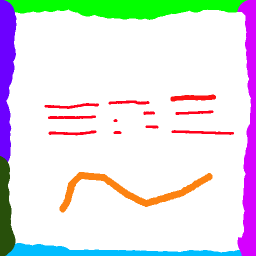$ | | ------------------------------------------------------------------------------------------------------------ | -------------------------------------------------------------------------------------------------------------- | |  |  | Instead of solving the system using a discretization of the domain and the operators, we will use a Monte Carlo integration process, mimicking path tracing in physically-based image rendering. # Warm-up 1. Update the repository and set up a project that would load an image ($g_0$) and output an image ($u$). 2. *Bruteforce Nearest Neighbors*: For each "white" pixel create a function to retrieve the index (and the distance) of the closest non-white one. 3. Output the image where each white pixel gets the color of its closest non-white pixel. :::info In the next lecture/practicals, we will discuss about efficient nearest-neighbor data structures. For this practical, let's consider a naive one and focus on the diffusion problem. ::: # The Walk-On-Sphere algorithm From the previous practical, we know that the solution of this elliptic PDE is harmonic. In other words, we have the following properties: at a point $x\in\Omega$, for any ball $B(x)$ centered at $x$, then **(Mean value property)** $$u(x)=\frac{1}{|\partial B(x)|}\int_{\partial B(x)} u(y) dy$$ The second key ingredient is the notion of **random walks**: Starting at $x$, if $w(y)$ is a random walk in $\Omega$ from $x$ that reaches some $y\in\partial\Omega$ (at each "step", the walker moves in a uniform random direction at a uniform random distance), then: $$u(x)= E[w(y)],\quad y\in\partial \Omega$$ (the value of $u$ at $x$ is the expected value of random walkers). 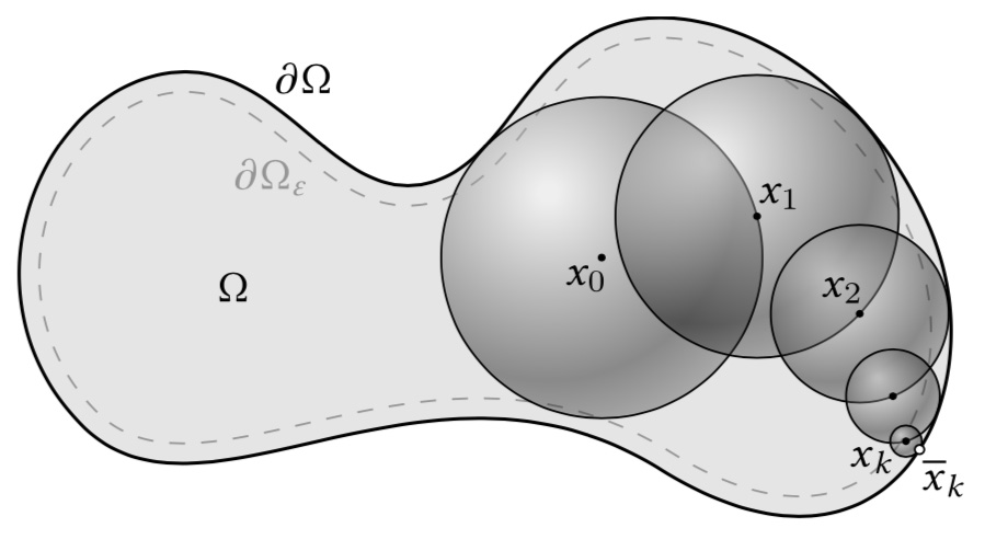Combining these ingredients, we can design a simple "path-based" Walk-on-sphere algorithm to evaluation $u(x)$ (without solving $u$ for all $x\in\Omega$)[^1]: a. Set $x_0=x$ b. For a given point $x_i$, compute the min distance $d$ to $\partial\Omega$ c. Draw a random point $x_{i+1}$ on $\partial B(x_i,d)$ (ball centered at $x_i$ with radius $d$) d. If $x_{i+1}$ is close to the boundary ($\epsilon$-close), retrieve the boundary conditions value $g(x_{i+1})$ e. Otherwise go to step b. This sketch generates a random path from $x$ to some $y=x_k\in\partial\Omega$:  To get the actual estimate $\tilde{u~}(x)$, we use a Monte Carlo approach to combine the integral and the expectation using discrete estimates. For short, $\tilde{u~}(x)$ is given by averaging $N$ random paths from $x$ to $\partial \Omega$. The parameters are thus: - The approximation parameter $\epsilon$. - The number of random path per point $x$ (denoted spp or $N$). - The *depth* of the path: if after $K$ steps, we haven't reached a point close to $\partial\Omega_\epsilon$, we just discard the path. The key point is that as the number of paths increases, the estimate $\tilde{u~}(x)$ converges to $u(x)$. | $g_0$ | 1spp | 16spp | 1024spp |4096spp | | ----- | 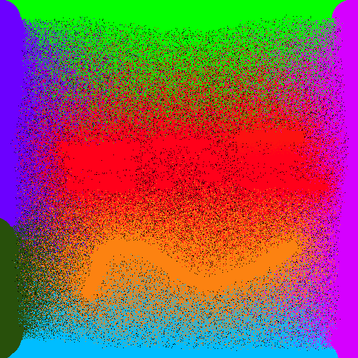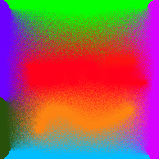---- | ----- | ------- |--------| |  |  |  |  |  4. Implement the Walk-on-Sphere algorithm using the white/non-white setting of the previous section ($\partial \Omega$ is the set of non-white pixels). The objective would be to estimate $\tilde{u~}(x)$ for each white pixel. ::: info As you will have to iterate over nearest-neighbor searches, I encourage you to cache the NN for each white pixel in a buffer. ::: 5. Once you have a first version of the code, experiment various spp and various depths. You can use your own image editor (MSPaint, Gimp..) to create various boundary conditions $g_0$. 6. For a single pixel, and for increasing spp (e.g. 1->4096 or more), plot the **variance** of the $\tilde{u~}(x)$ estimate as a function of the spp. As the Monte Carlo process being unbiased (only uniform samplers are used to construct the path), the **variance** plot should tend to zero. Use for instance `gnuplot` to plot the variance (in logscale). What is the convergence speed you are observing? # Few Monte Carlo tricks One of the most important features of this approach is its high versatility (no need to triangulate or discretize the domain) and the fact that we can rely on all path-tracing tricks using in image rendering to solve PDE (filtering, importance sampling, control variate, path reuse...). 7. Implement a simple reconstruction kernel whose idea is to get some raw values for low sample counts and then smooth them using some kernel (e.g. [Mitchell's filter](https://en.wikipedia.org/wiki/Mitchell–Netravali_filters)). 8. Instead of fixing the depth of the paths, you can implement a *Russian roulette* strategy (useful to explore unbounded domains as well): at each step, you flip a coin (Bernouilli test with some probability $q$) to decide whether you continue or not the path exploration. # References [^1]: Sawhney, Rohan, and Keenan Crane. "Monte Carlo geometry processing: a grid-free approach to PDE-based methods on volumetric domains." ACM Transactions on Graphics (TOG) 39.4 (2020): 123-1.