--- title: Statistics ---  <p><strong><span style="font-size: xx-large;">Statistics</span></strong></p> :::info École normale supérieure -- PSL, Département de biologie :mortar_board: [Maths training 2024-2025](https://codimd.math.cnrs.fr/s/hmbX8GuA4#) :bust_in_silhouette: Pierre Veron :email: `pveron [at] bio.ens.psl.eu` ::: Course inspired by Benoît Pérez-Lamarque and Jérémy Boussier [TOC] # Estimation ## What are statistics? **Probabilities** focus on predicting the outcome of experiments if the laws (distributions) of the outcomes are known: > If we toss a coin 10 times, what is the probability to obtain face 5 times? For **statistics**, it is the opposite: we want informations on the distributions given a realisation of an event. > We threw a coin 10 times and obtained face 6 times: can we say that the coin was balanced? Of course with only one realisation we can not conclude on the distribution the variable at the origin for sure, but we can reply, with a given margin of error, on several questions regarding the distribution of the variable. ## Some vocabulary * A **population** is the object of study. It is composed of individuals or objects that are assumed to be realisations $x_i$ of random variables $X_i$ that follow a common distribution $P_X$. * A **sample** is a finite subset of the population on which we can measure the characteristic. For instance we know the sample $x_1, x_2, ..., x_{10}$. * The **sampling** is the random selection of the individuals making up the sample. If the sampling is independant of the variables $X_i$ we say that the sampling is **unbiased**. If the sampling is conditionned on a given characteristic $A$ (for instance, only the individuals who agree to take part in a study. ) we no not estimate the distribution $P_X$ but $p_{X| A}$: the sampling is **biased**. ## Estimator Let $n$ be a positive integer, $X_1, ..., X_n$ independant random variables with the same distribution. This distribution depends on a parameter $\theta$ that is unknown. > For instance, $X_i = 1$ with probability $\theta \in (0,1)$ and $0$ otherwise ; $X_i$ follows a Bernoulli distribution with parameter $\theta$. An estimator $\hat \theta_n$ is a function of $X_1,...,X_n$ designed to estimate the true parameter $\theta$: \begin{equation} \hat\theta_n = f(X_1, ..., X_n). \end{equation} :::info Since an estimator is a function of $X_1, ..., X_n$ that are random variables, **an estimator is a random variable**. So it makes sense to calculate the distribution, expected value, variance... of an estimator. When running the experiment, we calculate the estimation on the sample: $u_n = f(x_1,...,x_n)$. Estimator = random variable. Estimation = unique realisation on this random variable, measured on the sample. ::: ## Properties of an estimator As we said, an estimator is designed to "estimate" the true parameter. To do so, it has to satisfy nice properties that make a "good estimator": :::danger **Unbiased estimator** (_Definition_) An estimator is unbiased if its expected value equals the parameter that we want to estimate: \begin{equation} E[\hat \theta_n] = \theta. \end{equation} ::: The difference between an estimator and the parameter value $E[\hat \theta_n] - \theta$ is called the bias, or error, of this estimator. :::danger **Convergent estimator** (_Definition_) An estimator is convergent or consistent if it converges to $\theta$ as the sample size increases: \begin{equation} \lim_{n\to\infty} \hat \theta_n = \theta. \end{equation} ::: _Remark._ If this convergence is in probability ($\forall \varepsilon,\ P(|\hat \theta_n - \theta | > \varepsilon) \to 0$) we say that the estimator is weakly consistent ; if this convergence is almost sure ($P(\lim_{n\to\infty} \hat \theta_n = \theta) = 1$), then we say that the estimator is strongly consistent. :::danger **Mean square error** (_Definition_) The **mean square error** of an estimator is: \begin{equation} \mathrm{MSE}(\hat \theta_n ) = E\left[ \left(\hat \theta_n-\theta\right)^2\right]. \end{equation} ::: _Remark._ If the estimator is unbiased, its MSE is its variance. ## Estimator of the expected value :::danger **Estimator of the expected value** (_Definition_) Let $X_1,...,X_n$ be iid random variables such that $E[|X_1|] < \infty$. We note $\mu := E[X]$ the true (unknown) expected value of this variable. The estimator of the expected value is the estimator defined as: \begin{equation} \overline{X}_n := \frac{X_1 + \cdots + X_n}{n} \end{equation} It is simply the empirical average of the sample. ::: $\overline{X}_n$ is an unbiased and convergent estimator of $\mu$. ## Estimator of the variance :::danger **Estimator of the variance** (_Definition_) Let $X_1,...,X_n$ be iid random variables such that $E[|X_1|] < \infty$ and $V(X_1) < \infty$. We note $\sigma^2$ the true unknowon variance of the variables. The estimator of the variance is defined as : \begin{equation} S_n^2 := \frac{1}{n-1} \sum_{i=1}^n (X_i - \overline{X}_n)^2 \end{equation} ::: $S_n^2$ is unbiased and convergent estimator of $\sigma^2$. We could be tempted to use the usual definition of the variance of the sample, ie the mean of the squared difference to the mean: \begin{equation} V_n = \frac{1}{n} \sum_{i=1}^n (X_i - \overline{X}_n)^2. \end{equation} However, this estimator is biased since $E[V_n] = \frac{n-1}{n} \sigma^2 \ne \sigma^2$. Taking $n-1$ instead of $n is called the Bessel correction and allows to remove this bias. :::info Intuition of the Bessel correction: this is due to the fact that a good estimator is based on $n$ independant observations (like the estimator of the expected value). However, when we calculated each residual $X_i - \overline{X}_n$ we do not have $n$ independant observations because the observations $X_i$ influence the value of $\overline{X}_n$. This is why the variations of $X_i - \overline{X}_n$ is a bit less than the variation of $X_i$. This difference is smaller when $n$ is large because each individual observation has a smaller weight in the estimation of the mean. ::: # Confidence intervals We are happy to have an unbiased and convergent estimator, but we would like to have a qualitative evaluation of its quality. To do so we want to know how fast an estimator converges to the parameter $\theta$ as the size of the sample increases. We also want to nkow what is **the probability of being wrong when we say that the estimator is close to its target**. That is where the confidence intervals are used. ## Definition :::danger **Confidence interval** (_Definition_) Let $\alpha \in (0,1)$ (the risk). Let $I_n$ an interval that is calculated as a functions of $X_1,...,X_n$. $X_n$ is an interval of confidence for the parameter $\theta$ with a level $1-\alpha$ if \begin{equation} P(\theta \in I_n) = 1-\alpha. \end{equation} The bounds of an interval of confidence are two random variables because they are functions of $X_1,...,X_n$. ::: We often chose the risk $\alpha = 5\%$. Using the definition, this would mean : if we sample a $n$ sample, we would have an interval $[A, B]$ such that the probability that $\theta$ is in $[A,B]$ is 0.95. The goal is to build the smallest interval possible which satisfies this condition. ## Example: normal distribution with known variance Let us assume that $X \hookrightarrow \mathcal{N}(\mu, \sigma^2)$ where $\sigma^2$ is known but $\mu$ is unknown. We have a sample $x_1,..., x_n$ that built from realisations of $n$ random variables iid $X_1,...,X_n$ following the same distribution as $X$. We use the estimator of the expected value $\overline{X}_n := (X_1+\cdots+X_n)/n$. The sum of independant normal variables is still a normal variable with the mean being the sum of the mean, and the variance being the sum of the variances (see the [probability course](https://codimd.math.cnrs.fr/s/k-RhvcpOv#222-Normal--gaussian-distribution)) so we can show that \begin{equation} Z_n := \sqrt{n} \frac{\overline{X}_n - \mu}{\sigma} \hookrightarrow \mathcal N (0,1) \end{equation} because $X_1 + ... + X_n \hookrightarrow \mathcal N(n\mu, n\sigma^2)$. Given a risk $\alpha \in (0,1)$, we look for a number $\beta>0$ such that \begin{equation} P(Z_n \in [-\beta, \beta]) = 1 - \alpha \end{equation} For instance, for $\alpha = 0.05, \beta \approx 1.96$. Now once we have $\beta$ we can also write that \begin{equation} -\beta \le Z_n := \sqrt{n} \frac{\overline{X}_n - \mu}{\sigma} \le \beta \quad \Leftrightarrow \quad \overline{X}_n - \frac{\beta \sigma}{\sqrt{n}} \le \mu \le \overline{X}_n + \frac{\beta \sigma}{\sqrt{n}}. \end{equation} So $I_n = [\overline{X}_n - \frac{\beta \sigma}{\sqrt{n}} ,\overline{X}_n + \frac{\beta \sigma}{\sqrt{n}}]$ is an interval of confidence of level $1-\alpha$ for the expected value $\mu$. ## Example: normal distribution with unknown variance Let us take the previous example but in this case the variance $\sigma^2$ is unknown. The interval of confidence is not working anymore. However we could substitute $\sigma$ to its estimator $S_n$, but in this case the variable $Z_n$ built with the observations is not normally distributed. Instead we have (admitted): \begin{equation} \sqrt{n} \frac{\overline{X}_n - \mu}{S_n} \hookrightarrow t(n-1) \end{equation} where $t(n-1)$ is Student's $t$ distribution with $n-1$ degrees of freedom. From the tables of values of the $t$ distribution, we can read $\beta$ such that \begin{equation} P\left( -\beta < \sqrt{n} \frac{\overline{X}_n - \mu}{S_n} < \beta \right) = 1-\alpha \end{equation} and thus deduce the interval of confidence: \begin{equation} P\left( \mu \in \left[\overline{X}_n - \frac{\beta S_n}{\sqrt{n}}, \overline{X}_n + \frac{\beta S_n}{\sqrt{n}}\right]\right) = 1-\alpha. \end{equation} # Hypotheses testing In this section, we are no longer interested in estimating parameters, but we want to anwer specific questions: > Does this drug has an effect? > Is cancer more likely in this population? > ... ## Vocabulary and notations Let us write the observations $x_1,...,x_n$, taken from random variables $X_1,...,X_n$ from unknown distributions. We introduce a statistics: \begin{equation} Y_n := f(X_1,...,X_n) \end{equation} and denote $y_n$ its realisation. * **Statistics**: quantity defined from the observations that is used for the test. 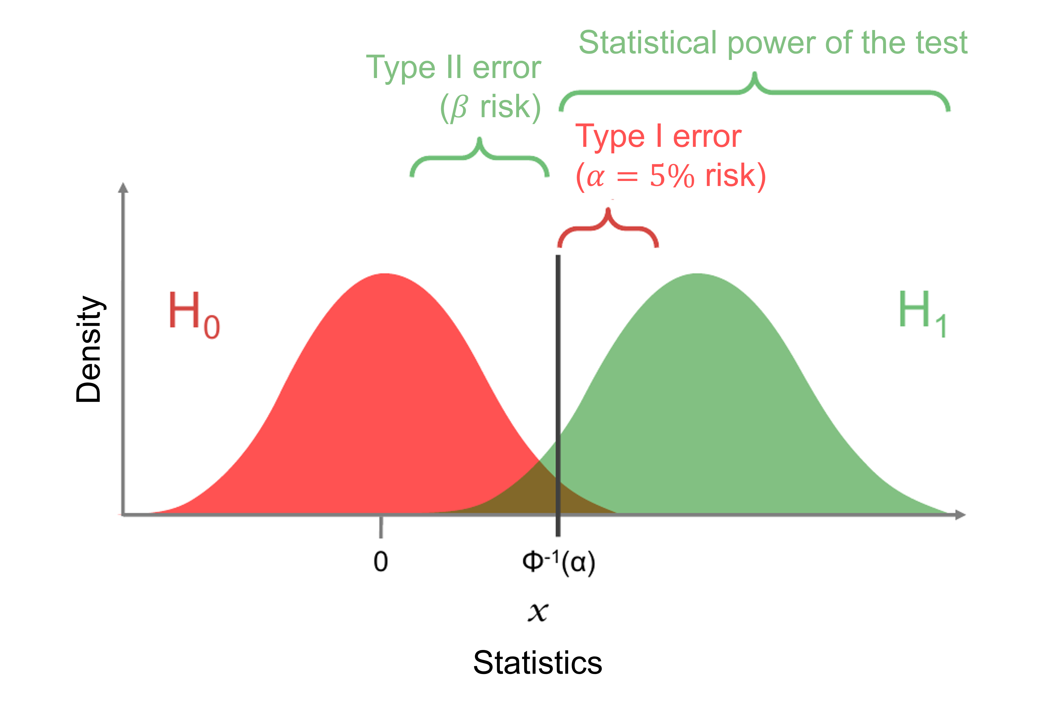* **Null hypothesis** $H_0$: hypothesis according to which the effect being studied does not exist. A positive answer to a statistical question is often a refutation of the null hypothesis. * **Alternative hypothesis** $H_1$ or $H_a$: hypothesis according to which $H_0$ is false. * **Reject zone** $W$: interval defined from the null hypothesis in which the statistics is not likely to be. If the statistics is in the reject zone, we reject the null hypothesis. * **Risk $\alpha$ or type I risk**: error of rejecting the null hypothesis if this hypothesis is true. We often take $\alpha = 0.05$. * **Risk $\beta$ or type II risk**: error of accepting the null hypothesis if this hypothesis is false. * **Statistical power**: ability to detect a difference when this difference exists, ie ability to reject $H_0$ when $H_0$ is false. The statistical power is $1-\beta$. * If the reject zone is a unique interval of the form $W = [\gamma, \infty[$ then we say the test is **unilateral**. If the reject zone is the union of two intervals, for instance $W = ]-\infty, -\gamma[ \cup ] \gamma, +\infty[$ then we say the test is **bilateral**. A hypothese testing is a test: 1. if $y_n \in W$ then we reject $H_0$ and accept $H_1$ 2. if $y_n \notin W$ then we do not reject $H_0$ nor $H_1$.  | ↓ Result of the test / Reality → | $H_0$ true | $H_0$ false | | -------------------------------- | ---------- | ----------- | | Non reject of $H_0$ | $1-\alpha$ | $\beta$ | | Reject of $H_0$ | $\alpha$ | $1-\beta$ | ## p-value The $p$-value is the probability, under $H_0$ that the statistics $Y_n$ takes a more extreme value than the realisation $y_n$. For unilateral testing, the $p$-value is : \begin{equation} P(Y_n > y_n | H_0) \end{equation} For bilateral testing, the $p$-value is: \begin{equation} P(|Y_n| > |y_n| \quad |\quad H_0). \end{equation} So: $H_0$ is rejected when $p \le \alpha$. ## Parametric or non-parametric test? A **parametric test** is a test for which a parametric hypothesis is made about the distribution of the data under $H_0$ (normal distribution, Poisson distribution, etc.). The hypotheses of the test then concern the parameters of this distribution. A **non-parametric test** is a test that does not require a hypothesis to be made about the distribution of the data. The data are replaced by statistics that do not depend on the means/variances of the initial data (contingency table, order statistics such as ranks, etc.). ## Quantitative or qualitative variable? A **quantitative variable** represents a quantity (time, temperature, size,...). It has value in $\mathbb R$ or a subset of $\mathbb R$ (for instance $\mathbb N$). A **qualitative variable** represents something that is not a quantity (example: blood type {A, B, AB, O}, or status {sick, not sick}, nationality, sex...). The values that this variable can take are called the levels of this random variables. ## In practice : how do we run a statistical test? 1. We fix a risk $\alpha$ (for instance 0.05) 2. We run $n$ experiments and note the results $x_1,...,x_n$. 3. We make hypotheses on the distributions that the variables $X_i$ follow (for instance $X_i$ follow a normal distribution) 4. We chose the null hypothesis $H_0$ and therefore the alternative hypothesis $H_1$. 5. We introduce a random variable, the statistics of the test $Y_n$ that is calculated as a function of the $X_i$ (for instance, the empirical average $(X_1+\cdots+X_n)/n$). 6. We calculate what is the distribution of $Y_n$ assuming $H_0$. 7. We deduce the reject zone $W$. 8. We calculate the realisation of $Y_n$, denoted $y_n$ based on the measured values $x_1,...,x_n$ 9. If $y_n$ is in the reject zone, we reject $H_0$ otherwise we do not reject it with a risk $\alpha$. 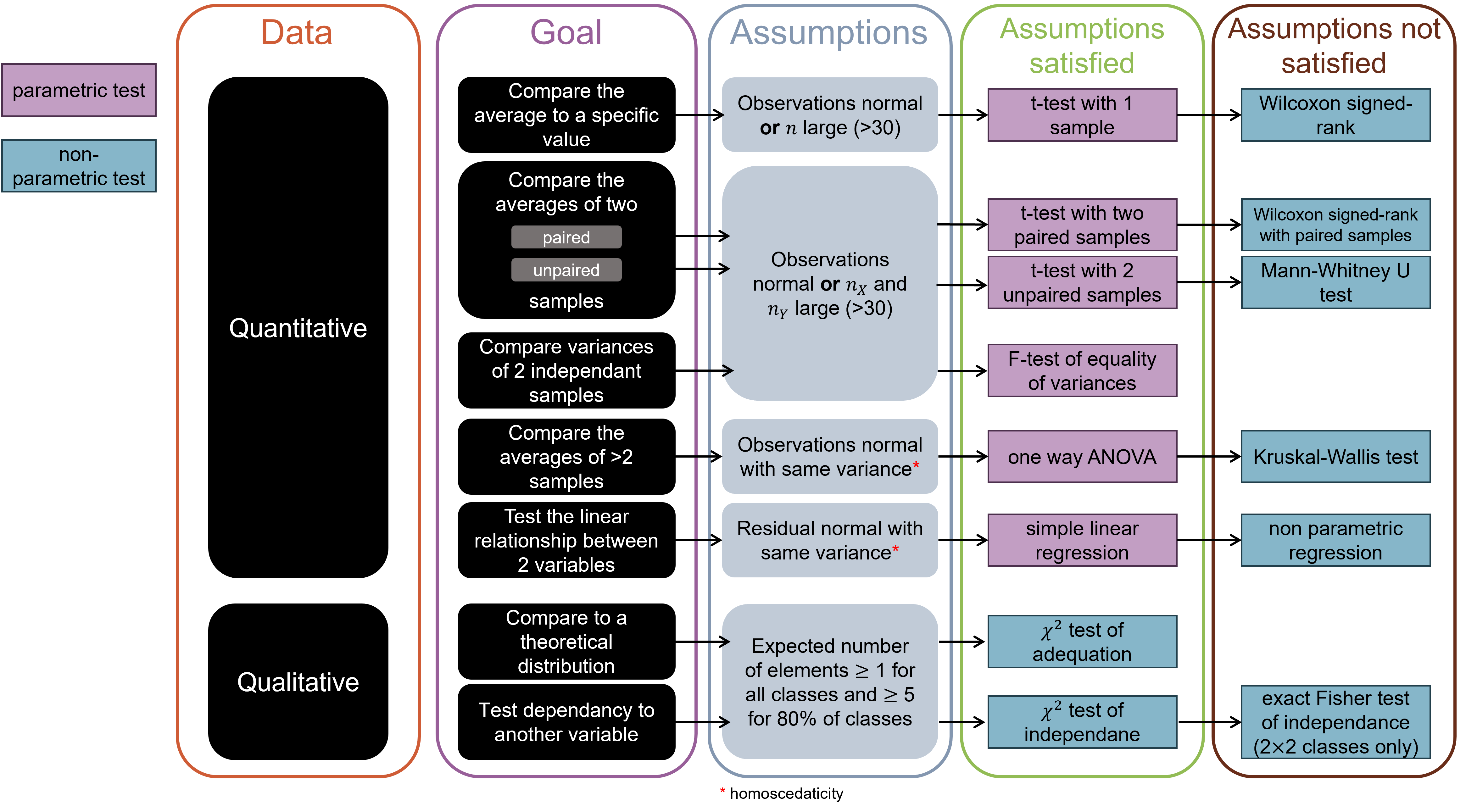# Usual tests ## Parametric tests for quantitative variables ### t-test with one sample :::info * **Assumptions** Let $X_1,...,X_n$ be iid random variables. We suppose that * either $X_i$ are normally distributed * or $n$ is large (typically $>30$). * **Null hypothesis**: $E[X_i] = \mu$ * **Test statistic**: $\sqrt{n} \frac{\overline{X}_n - \mu}{S_n}$ distributed under $t(n-1)$ if $H_0$ is true. * In `R` we can use the function `t.test(x=x, mu=mu, alternative="two.sided")` where `x` is the vector containing the observations, `mu` is the value to test, and `alternative` indicates whether we want to make a bilateral (`two.sided`) or unilateral (`less` or `greater`). ::: ### t-test with two paired samples :::info * **Assumptions** Let $X_1,...,X_n$ and $Y_1,...,Y_n$ be random variables such that: * $X_i$ are iid * $Y_i$ are iid * $X_i$ and $Y_j$ are independant when $i\ne j$ but $X_i$ and $Y_i$ can be dependant. We suppose that: * either $X_i-Y_i$ are normally distributed * or $n$ is large (typically $>30$). * **Null hypothesis** $E[X_i - Y_i] = 0 \Leftrightarrow E[X_i] = E[Y_i]$. * **Test statistic**: same as a $t$-test with one sample but with $\mu = 0$ and the variable $Z_i := X_i - Y_i$. If $H_0$ is true then this statistics is distributed under $t(n-1)$. * In `R`: use the function `t.test(x=x, y=y, paired=TRUE, alternative="two.sided")` or `t.test(x=y-x, mu=0, alternative="two.sided")`. ::: ### t-test with two unpaired samples :::info * **Assumptions.** Let $X_1,...,X_{n_X}$ and $Y_1,...,Y_{n_Y}$ be $n_X$ and $n_Y$ random variables such that: * $X_i$ are iid * $Y_i$ are iid * $X_i$ and $Y_i$ are independant. We suppose that: * $X_i$ and $Y_i$ are normally distributed * or $n_X$ and $n_Y$ are large (typically $>30$). * **Null hypothesis**: $E[X_i - Y_i] = 0 \Leftrightarrow E[X_i] = E[Y_i]$. * **Test statistic**: under $H_0$ the variable \begin{equation} Z_n := \frac{\overline X_n - \overline Y_n}{\sqrt{\frac{S_X^2}{n_X} + \frac{S_Y^2}{n_Y}}} \end{equation} follows a distribution $t(n_X+n_Y-2)$, with $S_X^2$ and $S_Y^2$ the unbiased estimators of the variance of $X_i$ and $Y_i$. * In `R`: `t.test(x=x, y=y, alternative="two.sided")`. ::: ### F-test of equality of variances (Fisher test) :::info * **Assumptions.** Let $X_1,...,X_{n_X}$ and $Y_1,...,Y_{n_Y}$ be $n_X$ and $n_Y$ random variables such that: * $X_i$ are iid * $Y_i$ are iid * $X_i$ and $Y_i$ are independant. We suppose that: * $X_i$ and $Y_i$ are normally distributed ($\mathcal N (\mu_X, \sigma_X^2)$ and $\mathcal N(\mu_Y, \sigma_Y^2)$). * or $n_X$ and $n_Y$ are large (typically $>30$). * **Null hypothesis**: the two variables have the same variance $V(X_i) = V(Y_i)$. * **Test statistic**: under the null hypothesis, the ratio of estimators of variances $S_X^2 / S_Y^2$ follows an $F$-distribution of $n_X$ and $n_Y$ degrees of freedom. * In `R`: `var.test(x=x, y=y, alternative = "two.sided")`. 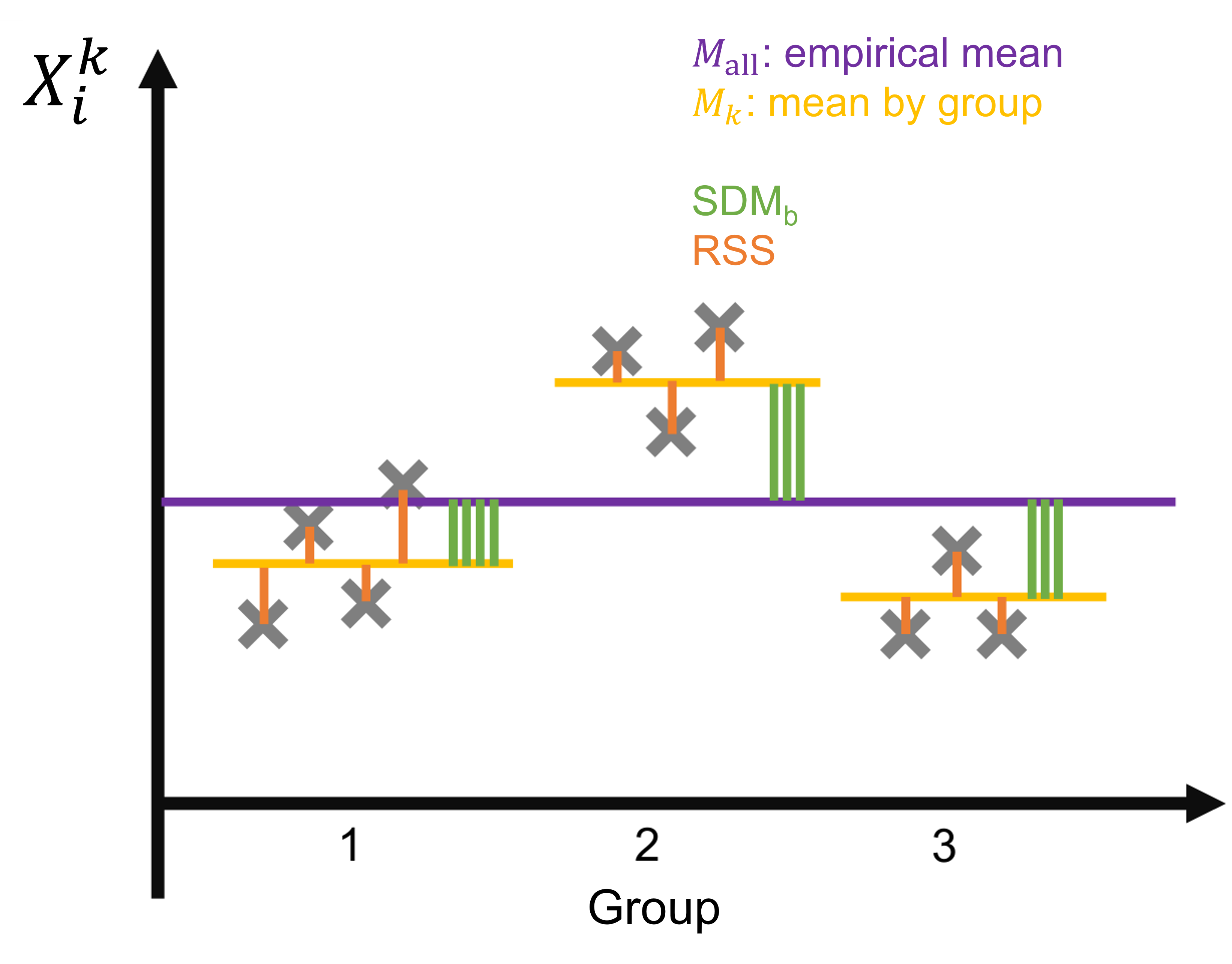::: ### One-way ANOVA :::info * **Assumptions** Let * $X_1^1, ..., X_{n_1}^1$ * $X_1^2, ..., X_{n_2}^2$ * ... * $X_1^p, ..., X_{n_p}^p$ be independant variables following normal distributions. We introduce $n := n_1 + \cdots + n_k$. We assume $\forall k = 1, ..., p$, $\forall i = 1,..., n_k$, $X_i^k \hookrightarrow \mathcal N(\mu_k, \sigma^2)$: all variables have the same variance (**homoscedaticity**). * **Null hypothesis**: all variables have the same expected value, ie $\mu_1=...=\mu_p$. * Test statistic: Let the between-group Squared deviations from the mean ($\mathrm{SDM}_b$) be the sum of the squared difference between the averages of the groups and the mean over all variables \begin{equation} \mathrm{SDM}_w = \sum_{k=1}^p n_k (M_k - M_{\mathrm{all}})^2 \end{equation} with $M_k = (X_1^k + \cdots + X_{n_k}^k) / n_k$ and $M_{\mathrm{all}} = (\sum_{k=1}^p \sum_{i=1}^{n_i} X_i^k) / n$. Let the residual sum of squares ($\mathrm{RSS}$) the sum of squared residuals between observations and their within-group mean: \begin{equation} \mathrm{RSS} = \sum_{k=1}^p \sum_{i=1}^{n_k} (X_i^k - M_k)^2. \end{equation} Then under $H_0$ we have: \begin{equation} F_n := \frac{\mathrm{SDM}_b/(p-1)}{\mathrm{RSS} / (n-p)} \hookrightarrow F(p-1, n-p). \end{equation} Intuitively, if the groups have the same mean, the SDM should be small compared to the RSS. * Function in `R`: `aov(y∼f, data=df)` where `df` is a dataframe with a column `y` containing the values $x_i$ and `f` is a factor containing the qualitative variables corresponding to the groups. :::  ### Standard linear regression Let us consider the iid variables $Y_1,...,Y_n$ coupled to the iid variables $X_1,...,X_n$. We assume that: \begin{equation} Y_i \hookrightarrow \mathcal N (\mu_i, \sigma^2) \quad \text{with} \quad \mu_i = a X_i + b \end{equation} We can determine the values of the estimators of $\hat a$ and $\hat b$ using the least squares method: denoting $y_i$ and $x_i$ the observations associated with the variables and $\varepsilon_i$ the random residuals: \begin{equation} \hat a, \hat b = \mathrm{arg} \min_{(a,b)} \left(\sum_{i=1}^{n} \varepsilon_i^2 \right) = \mathrm{arg} \min_{(a,b)} \left(\sum_{i=1}^{n} (y_i-ax_i-b)^2 \right) \end{equation} with this notation, $\varepsilon_i \hookrightarrow \mathcal N(0, \sigma^2)$. The null hypothesis is that $a=0$ and $b=0$ (two null hypotheses that can be tested separately). Statistics: \begin{equation} T_a = \frac{\hat a}{\mathrm{SE}(\hat a)} \quad \text{with the standard error} \quad \mathrm{SE}(\hat a) = \sqrt{S_n^2 \left(\frac{1}{n} + \frac{\overline X_n}{S_{xx}} \right)} \end{equation} and \begin{equation} T_b = \frac{\hat b}{\mathrm{SE}(\hat b)} \quad \text{with the standard error} \quad \mathrm{SE}(\hat b) = \sqrt{\frac{S_n^2}{S_{xx}}} \end{equation} where $S_n^2 = \sum_{i=1}^{n} \varepsilon_i^2 / (n-2)$ and $S_{xx} = \sum_{i=1}^{n} (X_i - \overline X_n)^2$. Under the null hypotheses: $T_a$ and $T_b$ follow a $t(n-1)$ distribution. _Interpretation in variance partitionning_. Let us define: * the **total** sum of squares \begin{equation} \mathrm{TSS} = \sum_{i=1}^n (Y_i - \overline Y_n)^2 \end{equation} * the **explained** sum of squares, ie the difference between the predicted value of $Y_i$ by the model and the mean of $Y_i$: \begin{equation} \mathrm{ESS} = \sum_{i=1}^n (\hat Y_i - \overline Y_n)^2 \end{equation} with $\hat Y_i = \hat a X_i + \hat b$ * and the **residual** sum of squares, ie the difference between the predicted value and the observed value of $Y_i$. \begin{equation} \mathrm{RSS} = \sum_{i=1}^n (Y_i - \hat Y_i) \end{equation} We have: \begin{equation} \mathrm{TSS} = \mathrm{ESS} + \mathrm{RSS}. \end{equation} The coefficient of determination ($R^2$) can be seen as the **proportion of variance that can be explained by the linear model**: \begin{equation} R^2 = \frac{\mathrm{ESS}}{\mathrm{TSS}} = 1 - \frac{\mathrm{RSS}}{\mathrm{TSS}}. \end{equation} :::info **Summary: linear regression** * Assumptions: * $X_i$ and $Y_i$ are continuous RV such that $Y_i = a X_i + b$ * the term of error in the observations $\varepsilon_i = y_i - ax_i-b$ are iid * $\varepsilon_i \hookrightarrow \mathcal N (0, \sigma^2)$ (normality and homoscedaticity of the residuals) * Null hypothesis * for $a$: $(H_0^a) \quad a = 0$ * for $b$: $(H_0^b) \quad b = 0$ * Statistics * $t$-tests with $n-2$ degrees of freedom (see before) * Function in `R` * `summary(lm(y ~ y, data = df))` with `df` a dataframe containing a column named `y` with the values of $y_i$ and a column named `x` with the values of $x_i$. * Interpretation * $R^2$ can be interpreted in terms of proportion of the variance that can be explained by the model. ::: ## Non-parametric tests for quantitative variables All the previously introduced tests require that the variables (or the residuals) follow a normal distributions (which is hard to check) or that the samples are large (which is not always the case). When it is not the case, we need to use **non-paramtric tests**. These test rely on the ranks of quantitative variables, instead of their averages, standard deviation... They have less statistical power than their parametric equivalent but should be chosen in a lot of case. | Comparison | Parametric test | Non-parametric test | Function on `R` | | ----------------------------- | -------------------------------- | -------------------------------------------- | ------------------------------------------- | | average of a sample | $t$-test with 1 sample | Wilcoxon signed-rank test | `wilcox.test(x=x, mu=mu)` | | 2 paired samples | $t$-test with 2 paired samples | Wicoxon signed-rank test with paired samples | `wilcox.test(x=x, y=y, paired=TRUE)` | | 2 independant samples | $t$-test with 2 unpaired samples | Mann-Whitney $U$ (or Wilcoxon rank-sum test) | `wilcox.test(x=x, y=y, paired=FALSE)` | | $p \ge 3$ independant samples | one way ANOVA | Kruskal-Wallis (or one-way ANOVA on ranks) | `kruskal.test(y~f, data=df)` | _Summary of usual non-parametric tests and their equivalent parametric test._ ## Test for qualitative variables Qualitative variables are meant to represent objects that can not be ordered or measured (not numbers). All the parametric and non parametric tests defined before make no sense for qualitative variables. ### χ2 test of adequation The $\chi^2$ test for categorial data ised used to compare a theoretical set size between categories to an observed one. > Example: The aim is to study whether the risk of developing a fever depends on the age group. We note the age group of 1,000 people selected at random from the French population who have had an episode of fever in the last 3 months: children, adolescents, adults or the elderly. The idea is as follows: it is assumed that being member of a certain age group for the 1,000 individuals with fever results from the realisation of qualitative random variables iid. $X_1, ..., X_1000$ with values in {child, teenager, adult, senior} (variable with $m = 4$ levels). The null hypothesis H0 to be tested is as follows: for any age group $x$, > \begin{equation} > P(X_i = x) = \text{proportion of invidials of this class in the population} > \end{equation} > We will then compare the theoretical numbers (theoretical proportions of children, teenagers, adults and seniors in the total population) and the observed numbers (observed numbers of children, teenagers, adults and seniors with fever). :::info Let $X_1,...,X_n$ iid random variables in a finite set ${a_1,...,a_m}$ with $m$ being the number of classes (or levels). * **Null hypothesis**: for any $j = 1,...,m$ and $i = 1,...,n$, $P(X_i=a_j) = p_i$ the _theoretical proportion_. We note \begin{equation} O_j = \#\{i, X_i = a_j\} \end{equation} the observed number of elements in class $j$. We introduce also: \begin{equation} E_j = p_j n \end{equation} the expected number of elements in class $j$. Note that this value can not be an integer. * **Test statistic**: Under the null hypothesis \begin{equation} U_n = \sum_{j=1}^m \frac{(O_j-E_j)^2}{E_j} \to \chi^2 (m-1) \quad \text{as} \quad n \to \infty \end{equation} Under $H_0$ the observed number of elements in a class is close to the expected one, so $U_n$ has to be close to 0. * **Assumptions**: the $\chi^2$ test is not exact but only asymptotic (true for $n$ large). To do so we have to check some "rule of thumb" assumptions: * for all $j$, $E_j\ge 1$ * 80% of classes must have $E_j \ge 5$. * In `R`: use the function `chisq.test(x = x, p = p)` where `x` is a vector containing the observed number of elements and `p` the expected probabilities $p_j$. ::: ### χ2 test of independance :::info * **Assumptions**: let $X$ and $Y$ be random variables with values in sets $\Omega_X=\{a_1,...,a_m\}$ and $\Omega_Y = \{b_1, ..., b_p\}$. We suppose that the expected number of elements per class $E_{j,k}$ is $\ge 1$ for all classes, and $\ge 5$ for 80% of classes. Let the contingency table be | ↓ $X=$ // $Y=$ → | $b_1$ | $b_2$ | ... | $b_p$ | | ---------------- | --------- | --------- | --- | --------- | | $a_1$ | $O_{1,1}$ | $O_{1,2}$ | ... | $O_{1,p}$ | | $a_2$ | $O_{2,1}$ | $O_{2,2}$ | ... | $O_{2,p}$ | | ... | ... | ... | ... | ... | | $a_m$ | $O_{m,1}$ | $O_{m,2}$ | ... | $O_{m,p}$ | Denoting $X_i$ and $Y$ the observations, for $i = 1,...,n$. With $\forall j,k$, $O_{i,j} = \# \{i, X_i = a_j, Y_i = b_k \}$. We also introduce the sums: $O_{+,k} = \sum_{j=1}^m O_{j,k}$, the number of observations such that $Y = b_k$, and $O_{j,+} = \sum_{k=1}^p O_{j,k}$, the number of observations such that $X = a_j$. The expected number of elements in the class $j,k$ is defined by: \begin{equation} E_{j,k} = \frac{O_{j,+}\times O_{+,k}}{n}. \end{equation} * **Null hypothesis** $X$ and $Y$ are independant, ie $\forall j, k$ \begin{equation} P(X = a_j\cap Y = b_k) = P(X = a_j) \times P(Y = b_k). \end{equation} * **Test statistics** Under the null hypothesis: \begin{equation} U_n := \sum_{j,k} \frac{(O_{j,k} - E_{j,k})^2}{E_{j,k}} \to \chi^2((m-1)(p-1)) \quad \text{as} \quad n \to \infty. \end{equation} * **Function in `R`**: `chisq.test(x = x)` where `x` is the contingency table, ie the table of observed number of elements $O_{j,k}$. ::: ### Exact Fisher test When the assumptions of the $\chi^2$ test are not met (small sample), and the contingency table is $2\times2$ (ie, $m=p=2$), there is an exact version of the test of independance called the exact Fisher test. In `R`, use the function `fisher.test(x)`, where `x` is the contingency matrix. ## Summary of usual tests  (c) Translated from Benoît-Perez Lamarque and Jérémy Boussier course. ## Multiple testing If we run 100 tests with a risk level of 5%, there is still ~5 cases where the test will be positive (reject the null hypothesis) by chance, even if the null hypothesis is true in all cases. With a $p$ risk level of $\alpha$, under the null hypothesis, the probability that at least one test among $n$ is positive is given by \begin{align} p_n &= P_{H_0} (\text{at least one $p$-value significant}) \\ &= 1 - P_{H_0} (\text{no $p$-value significant}) \\ &= 1 - (1 - \alpha)^n. \end{align} > For 2 tests, we have $p_2 \approx 0.1$, for 10 tests we have $p_{10} \approx 0.4$ and for 100 tests we have $p_{100} \approx 0.99$. In the last case we are almost sure to reject the null hypothesis in all situations. To solve this problem, there are 2 sulutions: 1. Either change the individual level of signifiance to keep a global level of signifiance of $\alpha = 0.05$ (for instnace). This is the Bonferroni correction (or FWER: family-wise error rate). A rule can be to divide the risk $\alpha$ by $n$, and reject the null hypothesis for one test only if $p < 0.05/n$. 2. Change the $p$-value (increase it artificially) to keep a level of individual signifiance of 0.05. This procedure is called FDR (false-disvoery rate): the obtained new $p$-values are called $q$-values. # Multivariate statistics: PCA Multivariate statistics is a branch of statistics interested in the distributions of variables in multidimensional spaces, for instance $\mathbb R ^d$. The methods involved in multivariate statistics aim at: * describing the information contained in high-dimensional data, * explain some variables by other variables. Multivariate statistics are more a form of data analysis (or data mining). Among these methods, the PCA (principal component analysis) allows to transform variables that are correlated into uncorrelated variables. In what follows, we will introduce the PCA. Let $\mathbf X = (X_1,...,X_n)$ be a random variable in $\mathbb R^n$. We introducve the covariance matrix: \begin{equation} \mathrm{Cov} (\mathbf X) = (\mathrm{Cov} (X_i, X_j))_{i,j} = \begin{pmatrix} V(X_1) &\mathrm{Cov}(X_1, X_2) & ... & \mathrm{Cov}(X_1,X_n) \\ \mathrm{Cov}(X_2,X_1) & V(X_2) & ... & \mathrm{Cov}(X_2,X_n) \\ \vdots & \vdots & \ddots & \vdots \\ \mathrm{Cov}(X_n, X_1) & \mathrm{Cov}(X_n, X_2) & ... & V(X_n) \end{pmatrix} \end{equation} where $\mathrm{Cov}(X, Y) = E[(X - E[X])(Y-E[Y])]$ is the covariance of two variables. Since $\mathrm{Cov}(X_i,X_j) = \mathrm{Cov}(X_j,X_i)$, the covariance matrix is symmetric. In particular, if $Z = \sum_{i = 1}^{n} u_i X_i = \mathbf{U}^{\intercal} \mathbf{X}$ is a linear combination of the variables $X_i$, with $\mathbf{U}^{\intercal} = (u_1,...,u_n)$ we have: \begin{equation} V(Z) = \sum_{i=1}^n \sum_{j=1}^n u_i u_j Cov(X_i, X_j) = \mathbf{U}^{\intercal}\mathrm{Cov} (\mathbf X) \mathbf{U}. \end{equation} Since $\mathrm{Cov} (\mathbf X)$ is real and symmetric, the spectral theorem says that it is diagonalizable in a orthonormal base, ie there is a base of $\mathbb R^n$ $\mathcal{B} = (\mathbf v_1, ..., \mathbf v_n)$ such that, \begin{equation} \forall i, \quad ||\mathbf{v}_i|| = \sqrt{\mathbf{v}_i^{\intercal} \mathbf{v}_i } = 1 \quad \text{and, }\forall j \ne i, \quad \mathbf{v}_i^{\intercal} \mathbf{v}_j = 0 \end{equation} in which the covariance is diagonal: \begin{equation} \mathrm{Cov} (\mathbf X) = P \begin{pmatrix} \lambda_1 & 0 & ... & 0 \\ 0 & \lambda_2 & ... & 0 \\ \vdots & \ddots & \ddots & 0 \\ 0 & 0 & ... & \lambda_n \end{pmatrix} P^{-1}. \end{equation} where $P$ is the matrix containing the coordinates of $\mathbf{v}_i$ as columns. Additionnaly, the eigenvalues $\lambda_i$ are positive since $\mathrm{Cov}(\mathbf{X})$ is a [nonnegative matrix](https://en.wikipedia.org/wiki/Nonnegative_matrix). We make the hypothesis that the eigenvalues are sorted in the decreasing order $\lambda_1 \ge \lambda_2 \ge cdots \ge \lambda_n \ge 0$. Let us consider the new variables, for $i = 1,...,n$: \begin{equation} Y_i = \sum_{j=1}^n v_{ij} X_j = \mathbf{v}_i^{\intercal} \mathbf{X} \end{equation} where $\mathbf v_i = (v_{i1},...,v_{in})$. More formally, the new multidimensionate variable $\mathbf{Y} = (Y_1,...,Y_n)^{\intercal}$ can be written $\mathbf Y = P \mathbf{X}$. Let us calculate the variance of $Y_i$: \begin{align} V(Y_i) &= \mathbf{v}_i^{\intercal} \mathrm{Cov}(\mathbf X) \mathbf{v}_i \\ & = \mathbf{v}_i^{\intercal} \lambda_i \mathbf{v}_i \quad \text{because $\mathbf v_i$ eigenvector} \\ & = \lambda_i \mathbf{v}_i^{\intercal} \mathbf{v}_i \\ & = \lambda_i \end{align} and similarly for $i \ne j$ \begin{align} \mathrm{Cov}(Y_i,Y_j) &= \mathbf{v}_j^{\intercal} \mathrm{Cov}(\mathbf X) \mathbf{v}_i \\ & = \mathbf{v}_j^{\intercal} \lambda_i \mathbf{v}_i \\ & = \lambda_i \mathbf{v}_j^{\intercal} \mathbf{v}_i \\ & = 0. \end{align} In summary: the transformed variable $\mathbf Y$ is a linear transformation of the variables $\mathbf{X}$ such that the components of $Y_i$ are uncorrelated and the variance of $V_i$ equals the eigenvalues of the covariance matrix. The variance of $Y_1$ is given by the largest eigenvalue, it is called the first axis of the PCA. It is the linear combination of $X_i$ that is orthogonal (norms is preserved) that maximises the variance. It can be seen as the direction on which the variance is maximal. The second axis is the linear combination, orthogonal to the first axis that maximises the remaining variance... That is why the PCA is commonly used to summarize data. *[iid]: independant and identically distributed *[RV]: random variables *[homoscedaticity]: property of variables having the same variances *[PCA]: principal component analysis