[CGDI] kd-Tree and MC Geometry Processing -bis-
===
> [name="David Coeurjolly"]
ENS [CGDI](https://perso.liris.cnrs.fr/vincent.nivoliers/cgdi/)
[TOC]
---
As you may have seen, the main bottleneck for the [last practical](https://codimd.math.cnrs.fr/s/b5SRBDUf0) was the efficiency of the nearest neighbors search. In this one, we will be playing with [kd-Tree](https://en.wikipedia.org/wiki/K-d_tree): a very efficient n-D data structure with $O(log(n))$ nearest-neighbor search.

::: warning
There is no code *per se* for this practical. The first section would only require a basic C++ or python file without any dependencies. For the last part of this practical, you would have to complete the code you wrote during the last practical.
:::
In dimension 2, the kd-tree algorithm can be sketched as follows:
```
BuildKdTree(S, depth)
if |S|=1
return a leaf containing this point
if depth is even
Retrieve the point p with median abscissa of S
Split S into two set according to the abscissa of p -> S1 and S2
if depth is odd
Retrieve the point p with median ordinate of S
Split S into two set according to the ordinate of p -> S1 and S2
SubTree1 = BuildKdTree(S1,depth + 1)
SubTree2 = BuildKdTree(S2,depth + 1)
return Tree(p , SubTree1, SubTree2)
```
In higher dimensions, we just have to split according to the point components, one-by-one, while increasing the depth value.
# Kd-Tree
Let's implement a first version of the kd-Tree in dimension 2.
1. Quick preliminary questions: what is the complexity of the median computation of an array of numbers? From that: what is the depth of the kd-Tree ? What is its number of nodes ? What is the computational cost of the kd-tree construction of $n$ points?
2. Implement the kd-Tree construction in dimension 2. For debugging purposes, you can create a function that traverses the tree (from the root to the leaves) and outputs the tree structure to the standard output.
E.g (using a breadth-first traversal):
```
> depth=0, median=val
>> depth=1, median=val'
>> depth=1, median=val''
...
...
>>>>>> depth=5, leaf, point=(0.3,0.4)
```
:::info
You can use `numpy.median` in python and `std::nth_element` in c++ for efficient median computations for random access vectors.
:::
4. By considering random 2d points in $[O,1)^2$, plot the experimental efficiency of your kd-tree construction as a function of $n$ (the number of points) ([matplotlib](https://matplotlib.org), [gnuplot](http://www.gnuplot.info)...)
The **nearest neighbor** of a point $p$ corresponds to a recursive traversal of the tree from the root while keeping the best NN: at each node, we first compare the current NN with the "median point" and update the best NN if needed. Then, we recurse on the subset containing $p$ (let say $S_1$), if the given best NN on $S_1$ has distance less than the distance to the medial line (*aka* the disk centered at $p$ touching the NN is fully contained in $S_1$), we just return this NN. Otherwise, we recurse on the second set $S_2$ and keep the best NN.
Here you have the illustration (initial setting, the NN on the left is fully contained on the left region so we do not need to check $S_2$, and the last case when the NN can be on both $S_1$ and $S_2$):

5. What is the worst-case complexity of the NN search on a tree with $n$ points.
6. Implement a **nearest neighbor** function and evaluate its experimental efficiency. For uniformly sampled points, you may observe an expected $O(\log{n})$ complexity of a single query. Evaluate and compare the efficiency of your NN search for other point distributions.
7. Now, let's consider a more unbalanced kd-tree construction in which the *split* is given by a random value. E.g. for an even depth, a random value between the max and min abscissa of $S$. Evaluate the efficiency of such approach in your uniform random sampling (as well as for a non-uniform one like non-centered Gaussian distribution).What do you observe? Please comment.
8. **extra** Update the code to construct a kd-tree in dimension 3 (with its nearest-neighbor search).
# Back to Monte Carlo Geometry Processing
Now that you have an efficient kd-tree structure, you can complete your [walk-on-sphere](https://codimd.math.cnrs.fr/s/b5SRBDUf0) implementation. Let me resketch the setting: you have a white image, some colored pixels and you would like to diffuse the color using a Lapace's equation.
For short, for a given white pixel $(i,j)$, the algorithms can be sketched as follows:
``` python
def solveLaplace(i,j)->(r,g,b):
r=g=b=0.0
cpt=0
x=i
y=j
for i from 0 to MAXSPP:
nbBounces=0
do
(k,l)<- getNearestNeighbor Pixel(x,y)
radius <- distance((x,y),(k,l))
(x',y') <- randomSampleOnCircle((x,y), radius)
(x,y) <- (x',y')
nbBounces++
while (radius > EPSILON) and (nbBounces < MAXDEPTH)
//if the final point is accepted, we retrieve the color
if (radius < EPSILON)
r += getRedColor(x,y)
g += getGreenColor(x,y)
b += getBlueColor(x,y)
cpt++
return (r/cpt, g/cpt, b/cpt)
```
9. Complete your Walk-On-Sphere algorithm using the kd-tree nearest-neighbor search using $n$ random colored samples in the image domain.
| | |
| -------- | -------- |
| 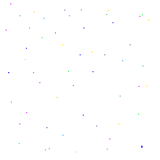 | 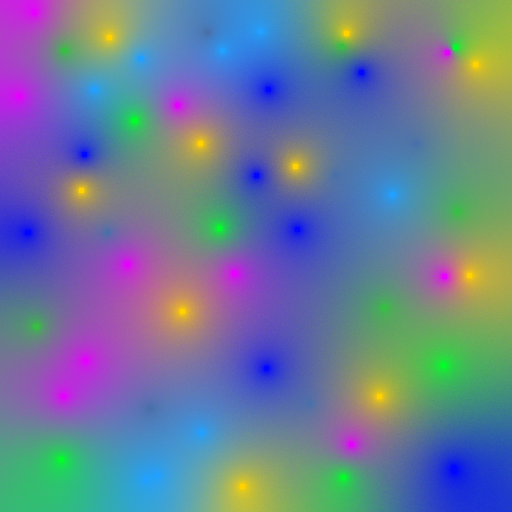 |