Practical: Digital Scale Axis
==
> David Coeurjolly
The objective of this practical is to implement a medial axis filtering technique called the scale axis[^1], using fast separable algorithms for the distance transformation and medial axis extraction. For this practical, the code skeleton is `practical-scaleaxis/scaleaxis.cpp` and it already contains the basic setup: the loading of a `vol`file and the visualization of its surface in [polyscope](https://polyscope.run).
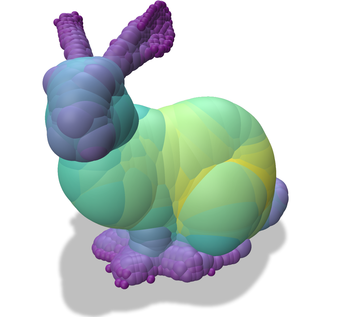
| Input Object | Medial Axis | Scale Axis |
| -------- | -------- | -------- |
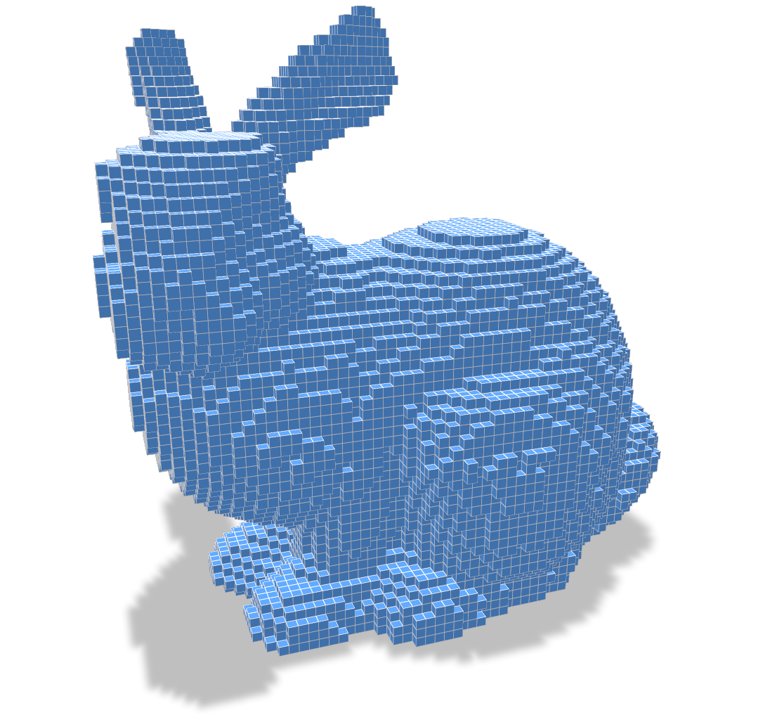 | 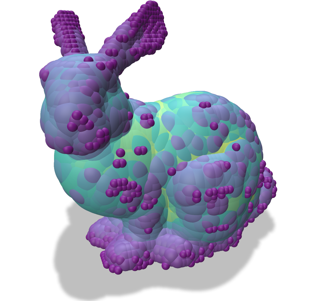 |
[TOC]
:::danger
:::spoiler Performances and multithread
When you code is up and running on small volumetric files, make sure to compile the project in cmake `Release` mode to get best performances (internal asserts will be disabled).
If you want to activate the parallel computation of the volumetric tools (distance transformation, medial axis, power map...), you would need an [openmp](https://openmp.org) enabled C++ compiler (most are compatible), and to have active this option in DGtal when you construct the cmake project. For instance, with the linux/macos command line:
```
cmake -DWITH_OPENMP=true -DCMAKE_BUILD_TYPE=Release ..
```
:::
Basic definitions (for a more formal setting, have a look to [^2] or [^3]):
:::success
:::spoiler Distance Transformation problem
Given a metric ($l_2$ here), label each point of an object with the distance to the closest background lattice point.
:::
:::success
:::spoiler Medial Axis problem
Given an input object and a metric, compute the set of maximal ball for the metric (balls inscribed in the object not included in any other inscribed ball).
:::
# Warm-up
In DGtal, we have an implementation of the [linear in time exact Euclidean distance transformation](https://dgtal-team.github.io/doc-nightly/moduleVolumetric.html) (or related problems such as the Voronoi diagram construction or medial axis extraction) for a large class of [metrics](https://dgtal-team.github.io/doc-nightly/moduleMetrics.html) using a (multithread) separable approach.
If you want to learn more, there is a [lecture available](https://perso.liris.cnrs.fr/david.coeurjolly/courses/voronoimap2d/).
1. Have a look to the documentation of the `DistanceTransformation` class. As you would see, to create a distance transformation instance, we need
* a domain (e.g. `Z3i::Domain` or the same domain as the input vol file `binary_image->domain()`)
* a predicate on grid points that returns true if the point is not a background point
* an instance of a separable metric (for instance `Z3i::L2Metric`).
When created, the `DistanceTransformation` instance is a model of an image containing the distance values for each point.
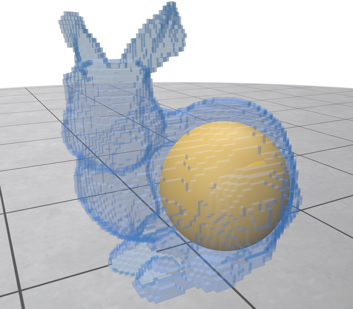
2. Compute the distance transformation of the input vol file and extract the largest inscribed ball
:::info
In polyscope, balls can be visualized using a [PointCloud](https://polyscope.run/structures/point_cloud/basics/) structure for which radius values are stored in a scalar quantity attached to points. For instance
```c++
std::vector<Z3i::Point> pointcloud;
std::vector<double> pointcloudRadii;
pointcloud.push_back( Z3i::Point(1,2,3));
pointcloudRadii.push_back(10.0);
pointcloud.push_back( Z3i::Point(3,1,2));
pointcloudRadii.push_back(20.0);
auto ps = polyscope::registerPointCloud("Two balls", pointcloud);
auto q = ps->addScalarQuantity("radii", pointcloudRadii);
ps->setPointRadiusQuantity(q,false);
```
creates (and display) a new structure with two balls with radii 10.0 and 20.0
:::
You should get something like this (with transparency in polyscope):
3. Display all inscribed balls centered at each interior points (not necessarily maximal ones).
:::warning
Depending on your GPU, displaying millions of spheres in a OpenGL context (polyscope) may not be a great idea.. Just test on small vol files.
:::
To compute the Medial Axis, we use the power map approach as described in [^3]: Given a set of inscribed balls (for example the output of the distance transformation), if we compute the power map (Voronoi diagram with additive weights corresponding to the square of the ball radii), maximal balls corresponds to power map sites with empty cells (when restricted to the input shape). To extract the medial axis, we first need to compute an image with squared radii. If `distance` is the distance transformation instance, the following snippet creates this new image:
```c++
ImageContainerBySTLVector<Z3i::Domain, DGtal::uint64_t> squaredDT(distance.domain());
for(auto p: distance.domain())
squaredDT.setValue(p, (p-distance.getVoronoiSite(p)).squaredNorm());
```
Now, you can create an instance of the [PowerMap](https://dgtal-team.github.io/doc-nightly/classDGtal_1_1PowerMap.html) class using this squared distance map. Then, the [ReducedMedialAxis](https://dgtal-team.github.io/doc-nightly/structDGtal_1_1ReducedMedialAxis.html) will extract the maximal balls (non-empty cells of the power map) as an image (non-zero values correspond to the square of balls radii centered at that point).
4. Compute and display the reduced medial axis of the input shape.
# Scale Axis
The objective of the scale axis is to filter the set of maximal balls in order to have a smaller set of balls that represent as much as possible the input object geometry. The idea is, from that filtering parameterized by a scalar parameter, to construct an approximated medial axis that is more stable and robust to noise.
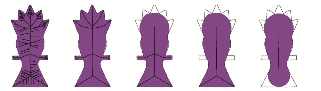
(image from [^4])
The algorithm is quite simple, given a scale parameter $s$ and a collection of balls (original medial axis)
* scale by $s$ the medial axis ball radii
* compute the union of these *inflated* balls
* extract the medial axis of that shape
* return the balls with radii scaled by a factor $1/s$
When transposed into the digital domain, it becomes even more trivial:
* Compute the distance transformation
* Scale the DT values by a factor $s$
* Compute the squared distance image and its power map
* return the ReducedMedialAxis balls scaled by $1/s$
:::danger
:::spoiler Complexity
For an input 3d object in an $[0,n-1]^3$ domain, the distance transformation, the power map and the medial axis extraction are linear, for the $l_2$ metric, in the number of grid points (i.e. $O(n^3)$ here). The scale axis transform for a given scale factor will have the exact same complexity.
:::
6. Implement the digital scale axis transform.
:::info
In the code skeleton, we have already set a slider and a variable to store the scale factor, and a button to launch the main computation.
:::
# References
[^1]: Giesen, Joachim, et al. "The scale axis transform." Proceedings of the twenty-fifth annual symposium on Computational geometry. 2009.
[^2]: Rosenfeld, Azriel, and John L. Pfaltz. "Distance functions on digital pictures." Pattern recognition 1.1 (1968): 33-61.
[^3]: Coeurjolly, David, and Annick Montanvert. "Optimal separable algorithms to compute the reverse euclidean distance transformation and discrete medial axis in arbitrary dimension." IEEE transactions on pattern analysis and machine intelligence 29.3 (2007): 437-448.
[^4]: Miklos, Balint, Joachim Giesen, and Mark Pauly. "Discrete scale axis representations for 3D geometry." ACM SIGGRAPH 2010 papers. 2010. 1-10.