[CGDI] Geometry Processing: Discrete Differential Operators on Meshes and Dirichlet Problems === > [name="David Coeurjolly"] ENS [CGDI](https://perso.liris.cnrs.fr/vincent.nivoliers/cgdi/) [TOC] --- In this lecture, we will be playing with differential estimators and solving PDE on meshes, such as Poisson based geodesics:  ::: info For this practical, you would need either a `c++` and a `python` to load an OBJ and circulate on a manifold mesh structure (cf Practical 4). ::: # Basic Differential Operators Let us consider the class of piecewise smooth linear functions defined at the mesh vertices. More precisely, the value at a point $p$ with barycentric coordinates $\{\phi_i, \phi_j,\phi_k\}$ in the triangle $t_{ijk}$ is $$ f(p) = f_i \phi_i + f_j \phi_j + f_k\phi_k\,.$$ where $\{f_i, f_j,f_k\}$ are the function values at vertices $i,j,k$. :::success This corresponds to considering classical "hat" basis functions from conformal [Finite Element Methods](https://en.wikipedia.org/wiki/Finite_element_method). ::: 1. **Warm-up** Create a simple code that opens an OBJ file (*e.g.* `spot.obj`) and assigns to each vertex, a scalar value depending on the vertices positions (as a linear or trigonometric function of the vertex positions). This will be your $\{f_i\}$ function. *E.g.*: | Linear | Sin | | -------- | -------- | | 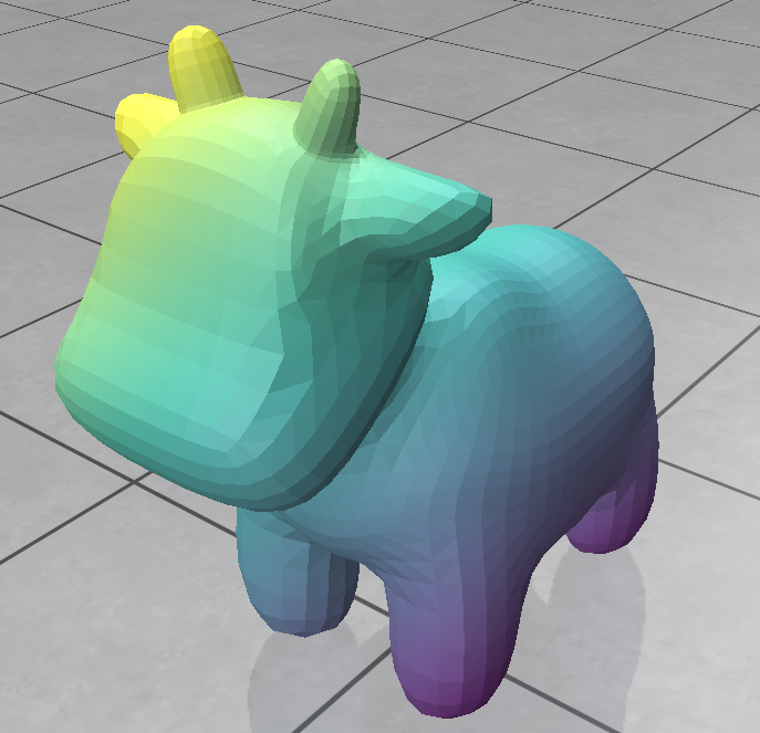 | 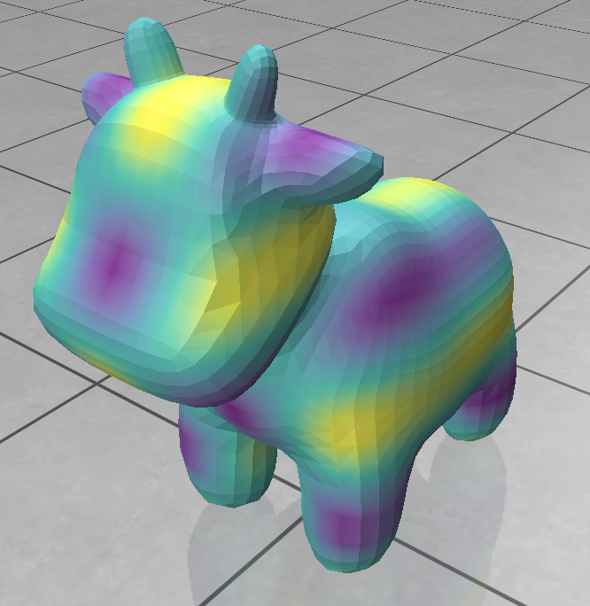 | ::: info Just use a `addVertexScalarQuantity`/`add_scalar_quantity` and let polyscope linearly interpolate on the faces? ::: One the most basic operators on scalar functions is the gradient. As the function being piecewise linear on the faces, we expect a constant gradient per face (aka **vertex-based gradient**) given from the gradient of the basis functions $\nabla\phi_i$: $$ \nabla f(p) = f_i \nabla\phi_i + f_j \nabla\phi_j + f_k\nabla\phi_k\,.$$ with $$ \nabla \phi_i := \frac{1}{2 a_{t_{ijk}}} \left(\vec{n~}_{ijk}~\times \vec{e~}_{jk}\right)$$ ($a_{t_{ijk}}$ is the area of the triangle, $\vec{n~}_{ijk}$ is normal vector and $\vec{e~}_{jk} := (x_k - x_j)$ the *edge vector*). 2. Compute the necessary quantities (or retrieve them from the API): the area and the normal vector for each triangle. 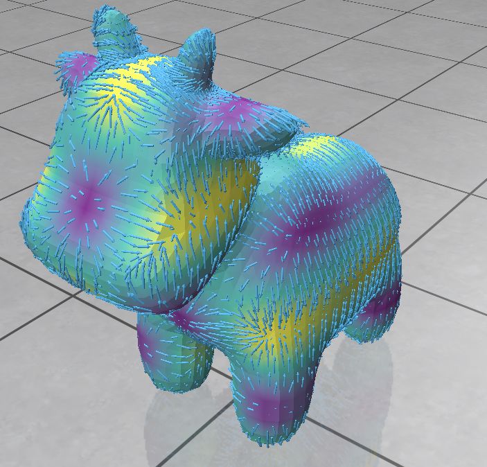3. Write a function that, for each triangle, its area, its normal vector and the three values $\{f_i, f_j,f_k\}$, computes the per face gradient of $f$ (and attach it to the geometry as a `FaceVectorQuantity` in `polyscope`). You should get something like:  On instrinsic vector fields, two extra quantities will be needed: the [divergence](https://en.wikipedia.org/wiki/Divergence) ("$\operatorname{div}$" or "$\nabla\cdot$") and the [curl](https://en.wikipedia.org/wiki/Curl_(mathematics)) ("$\operatorname{curl}$" or "$\nabla\times$") . For short, the divergence is a scalar value that measures how a vector field converges or diverges (it accounts to sinks and sources). The curl measures how the vector field *rotate* in a given neighborhood. :::info Any vector field can be decomposed into a divergence-free part, a curl-free one and a harmonic part (aka [Helmholtz-Hodge decomposition of VF](https://en.wikipedia.org/wiki/Helmholtz_decomposition)):  ::: In the setting of the practical (2D discrete triangular surfaces embedded in $\mathbb{R}^3$), one can discretize the divergence and curl at vertex $v_i$ of a per-face vector field $U$ as: $$\operatorname{div}(U)_i = - \sum_{t_{ijk}\supset v_i} \vec{u~}_{ijk}\cdot (\vec{n~}_{ijk}\times\vec{e~}_{jk}) $$ and $$\operatorname{curl}(U)_i = \sum_{t_{ijk}\supset v_i} \vec{u~}_{ijk}\cdot \vec{e~}_{jk} $$ ::: success **Note**: From vector caclulus, the curl is a vector. In our setting, 2d surface embedded in $\mathbb{R}^3$ and curl of intrinsic vector fields, the above scalar formula corresponds to the norm of the curl which is in the direction of the normal vector. ::: 4. Compute and display the divergence of $\nabla f$. The divergence must be positive on *sources* and negative on *sinks*. :::info For gradient of scalar functions $f$, we have $\operatorname{curl}(\nabla f) = 0$. ::: 5. **extra** As a sanity checks, you can verify the basic fundamental properties on calculus: $$ \operatorname{div}(U) = \operatorname{curl} Rot U\quad $$ ($Rot \vec{u~}_{ijk} := \vec{n~}_{ijk}\times \vec{u~}_{ijk}$, rotation of a vector field by 90 degrees -anti-clockwise for outward normal vectors- around the normal vector.) ::: success **Note** that these basic operators can be nicely extended to polygonal meshes (non-convex, non planar faces) [^1]. ::: ::: info The divergence operator will be used in the last part of the practical. ::: # Laplace-Beltrami From the above-mentioned operators, one can define the [Laplace-Beltrami](https://en.wikipedia.org/wiki/Laplace–Beltrami_operator) operator as $\Delta f:= - \operatorname{div}(\nabla f)$. On triangular meshes, we end up with the classical "cotan" Laplace-Beltrami operator as a linear operator on vertices $V$ (aka matrix $|V|\times |V|$). Its **weak form** is $$ L_{ij} = \left\{ \begin{array}{l} -\omega_{ij}\quad\text{$ij$ is an edge}\\ \sum_{k\in N(i)} \omega_{ik}\quad\text{$i=j$}\\ 0 \quad\text{otherwise} \end{array}\right . 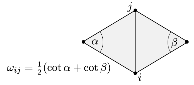$$ with  If $M$ denotes the $|V|\times |V|$ **mass matrix**, the diagonal matrix where $M_{ii}$ is the **vertex area** of the vertex $i$. There are several ways to define this vertex area. For the sake of simplicty for the practical, we can simply consider one third of the sum of adjacent triangle areas: $$ M_{ii} = \sum_{f\supset v_i} \frac{1}{3} Area(f)$$ We then define $\Delta_{cotan} = M^{-1}L$. :::info Note that some PDE formulations on meshes may only consider the *weak* for of the Laplace-Beltrami operator (see below). ::: 6. In a `numpy array`, `scipy sparse matrix`, or an `Eigen::MatrixXd` (or even better, a [Sparse Matrix](https://eigen.tuxfamily.org/dox/group__TutorialSparse.html)), implement the Laplace-Beltrami operator on triangular meshes. Make sure that all rows and columns sum up to zero. For some scalar functions of question 1, compute and show $\Delta_{cotan} F$ ($F$ being the vector of size $|V|$ containing $\{f(v_i)\}_{v_i\in V}$, the product is a vector defining a vertex scalar quantity). $E.g.$ the Laplacian must be zero on linear functions. We would like to use the Laplace-Beltrami opertator to solve [Dirichlet problems](https://en.wikipedia.org/wiki/Dirichlet_problem) on meshes. For instance, related to the [Laplace's equation](https://en.wikipedia.org/wiki/Laplace%27s_equation), we want to find $f$ such that: $$\begin{align} \Delta u &= 0\\ &s.t.\,\, u =g_0 \text{ on } \partial \Omega \end{align} $$ For short, some values are given at the boundary of a mesh ($g_0$) and we want to *diffuse* the values to remaining vertices. As $\Delta_{cotan}$ is a linear operator represented as a (sparse) matrix, solving the Laplace's equation corresponds to solving a linear system $Ax=b$. 7. Using `numpy` (e.g. [doc](https://numpy.org/doc/stable/reference/generated/numpy.linalg.solve.html)), `scipy` (e.g. [doc](https://docs.scipy.org/doc/scipy/reference/generated/scipy.sparse.linalg.spsolve.html#scipy.sparse.linalg.spsolve)), `eigen` ([doc](https://eigen.tuxfamily.org/dox/group__TutorialLinearAlgebra.html)), or `geometry-central` wrapper (e.g. [doc](https://geometry-central.net/numerical/linear_solvers/)) linear algebra solver, implement a Lapalce's equation solver on the `bunnyhead.obj` object (you would have to set some smooth values on the vertices boundary, cf previous practical). ::: info For higher efficiency, you can consider sparse matrices and sparse solvers. Note that $\Delta_{cotan}$ is Positive Semi-Definite (PSD) for which very efficient pre-factorization based solvers can be used. ::: You should get something like that: | $g_0$ | $u$ | | ----- | ---- | |  |  | ::: info For Laplace problems: solving $\Delta_{cotan}u=0$ $\Leftrightarrow$ $Lu=0$. For [Poisson problems](https://en.wikipedia.org/wiki/Poisson%27s_equation), solving $\Delta_{cotan}u=f$ $\Leftrightarrow$ $M^{-1}Lu=f$ $\Leftrightarrow$ $Lu=Mf$. So, no need to inverse the mass matrix and we can keep it sparse. ::: :::warning **Warning**: When discretizing the problem boundary conditions should taken carefully into considrection. For instance, as $u$ is fixed to values $g_0$ at some vertices, the Dirichlet boundary condition setting would make the boundary vertices to be removed from the linear problem ($i.e.$ some rows/cols of $L$ must be removed). We won't go into the details for this practical but just be aware of that. ::: ::: success The resulting function $u$ has very nice properties as $u$ is [harmonic](https://en.wikipedia.org/wiki/Harmonic_function) (smooth, mean value property,...). ::: # Geodesic in Heat At this point, we have some basic operators, the Laplace-Beltrami one (which is the Swiss army knife for many geometry processing algorithms), and already solved a first basic, yet fundamental, elliptic PDE. We would like now to estimate geodesic on meshes and for that, we will use the heat kernel approach[^2]. The intuition is the following one: you heat up the surface at given point $x_0$ and you measure the temperature at another point $y$ (at a given time $t$). The heat flow follows the [heat diffusion equation](https://en.wikipedia.org/wiki/Heat_equation) $$ \frac{\partial k_{t,x_0}}{\partial t} = \Delta k_{t,x_0} $$ Then the geodesic distance between $x_0$ and $y$ (known as Varadhan's formula): $$ d(x_0,y) = \operatorname{lim}_{t\rightarrow 0} \sqrt{-4t\log(k_{t,x_0}(y))}$$ We can thus solve the heat equation using an Euler scheme for instance, and then to take the $log$ of that function to get the distance. However, this turns out to be highly numerically unstable. In the following we will be considering the **Geodesic in Heat**[^2] approach which involves three steps: * First, we solve the heat equation for $u$ such that $\dot{u}=\Delta u$, for small $t$ using a single step backward Euler. * Construct the vector field: $X = -\nabla u/\|\nabla u\|$. * Solve the Poisson equation $\Delta \phi = \operatorname{div}(X)$. The intuition is that values of $u$ are not reliable but its gradient is. Then, we are looking for the smoothest function $\phi$ that matches with the sinks/sources of the normalized vector field (its divergence). 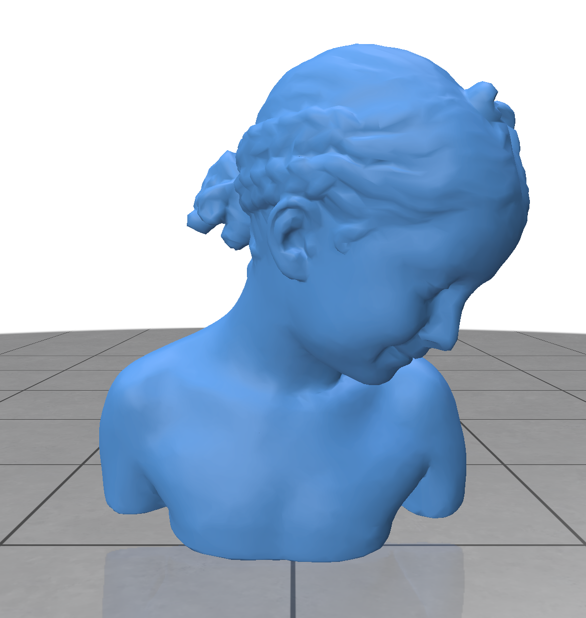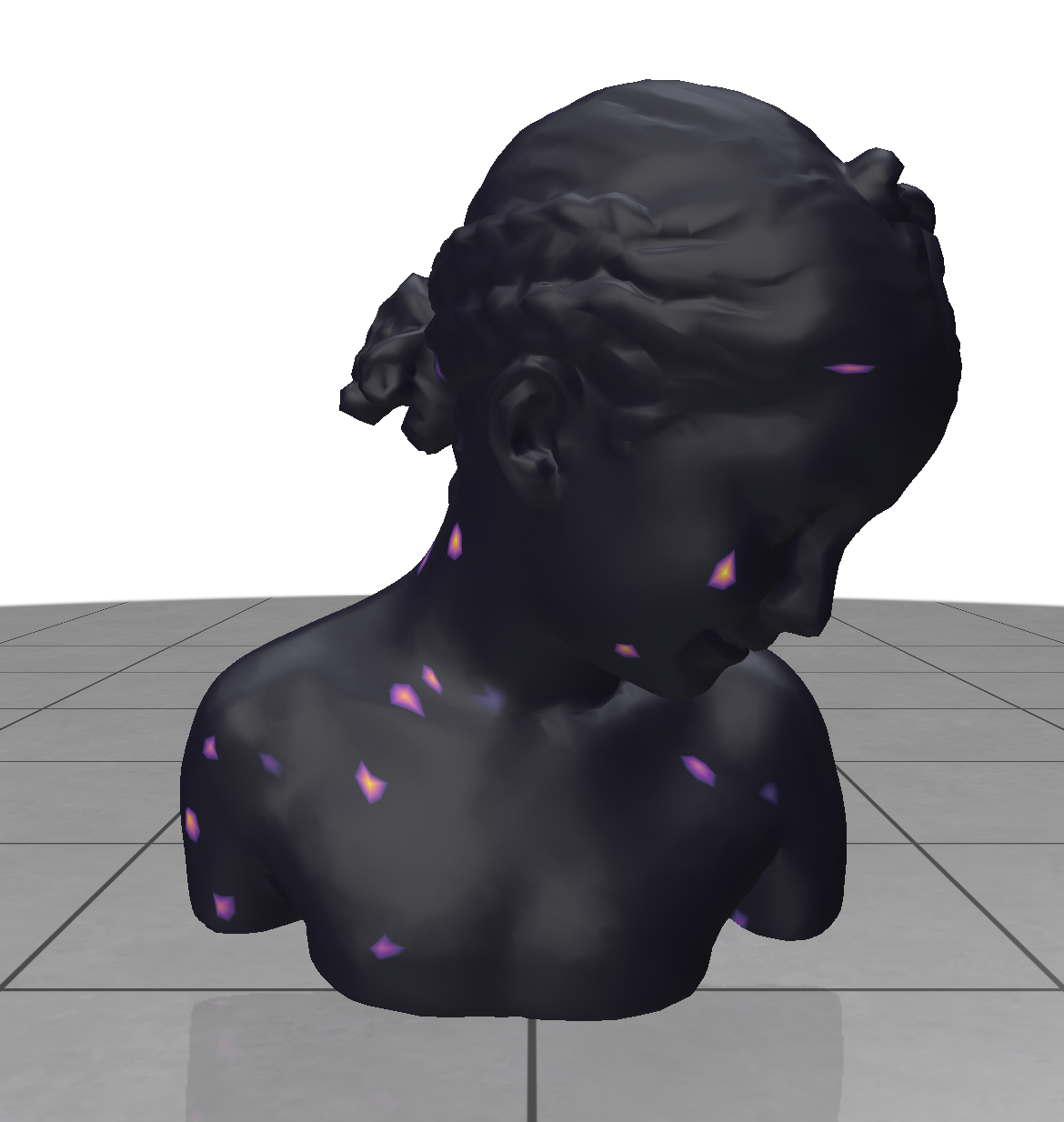8. Compute and display the solution of the heat equation by solving: $$ (M + t L)U = MU_0$$ ($U$ is a $|V|$ vector, $U_0$ is a null vector except at source vertices --`1.0` for instance--). ::: warning **Few details on the backward Euler**: to solve $\dot{u}=\Delta u$, we discretize the time and use the backward Euler scheme in $t$: $u(t+1) = u(t) + t\Delta u_{t+1}$. By stability of this scheme, we can do a single step approximation with: $$ u_t= u_0 + t\Delta u_t$$ Leading to $$ (I - t\Delta)u_t = u_0$$ Once discretized with $-\Delta \approx M^{-1}L$, we end up with $$(M + tL)U = MU_0\,.$$ ::: 9. Compute and display $\nabla u$, $X$ and $\operatorname{div}(X)$. 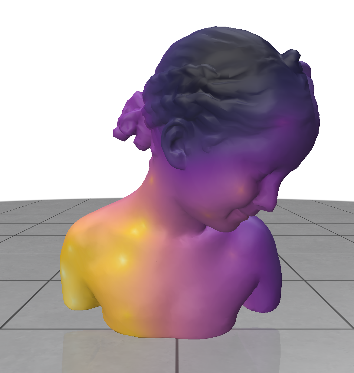10. Complete the overall **Geodesic in Heat** approach to compute $\phi$. 11. Experiment your code for various (but small) values of $t$. 12. If now we want to change the source vertex $x_0$ in $U_0$, what we would have to update in the algorithms? :::info **Few hints:** * As for the Laplace problem, you'd need a fast-linear solver on Sparse Matrix from either `eigen` or `numpy`. For non-degenerate triangulation $\Delta_{cotan}$ is Positive semi-definite (PSD) which admists fast prefactorized solvers for sparse matrix. 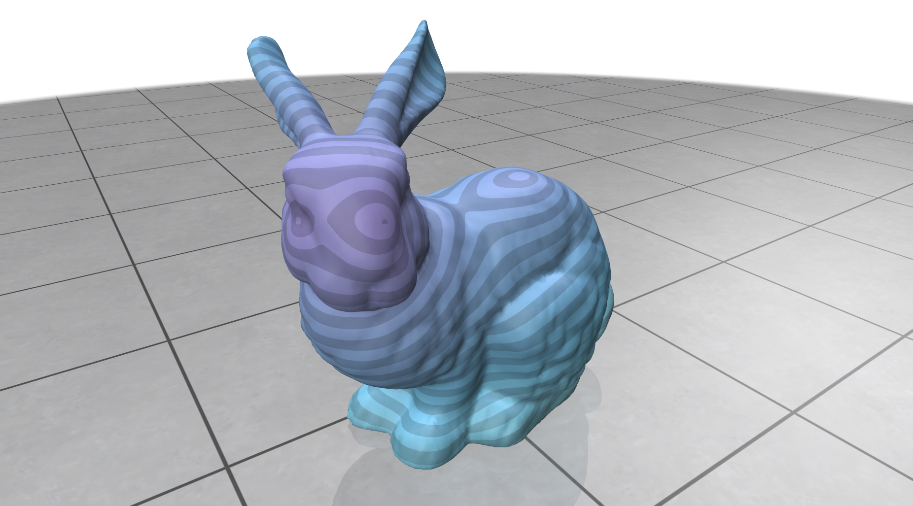* In `polyscope`, distances can be displayed using a dedicated distance quantity (cf [[c++]](https://polyscope.run/structures/surface_mesh/distance_quantities/), [[python]](https://polyscope.run/py/structures/surface_mesh/distance_quantities/)) with nice isolines shader. * You can add as many sources as you want in $U_0$. ::: and *voilà*...  [^1]: De Goes, Fernando, Andrew Butts, and Mathieu Desbrun. "Discrete differential operators on polygonal meshes." ACM Transactions on Graphics (TOG) 39.4 (2020): 110-1. [^2]: Crane, Keenan, Clarisse Weischedel, and Max Wardetzky. "Geodesics in heat: A new approach to computing distance based on heat flow." ACM Transactions on Graphics (TOG) 32.5 (2013): 1-11.