---
title: INFO001 (8b) Apprentissage supervisé
type: slide
slideOptions:
transition: slide
progress: true
slideNumber: true
---
# Apprentissage supervisé
## (Traitement et Analyse d'Image 8b)
>
> [name=Jacques-Olivier Lachaud][time=Decembre 2020][color=#907bf7] Laboratoire de Mathématiques, Université Savoie Mont Blanc
> (Les images peuvent être soumises à des droits d'auteur. Elles sont utilisées ici exclusivement dans un but pédagogique)
###### tags: `info001`
*(Some illustrations taken from S. Prince, Understanding Deep Learning, 2025)*
---
## Apprentissage et approximation

:::info
Apprentissage spécifique à un problème donné, approximation ou classification
:::
==base d'apprentissage== $N$ données $(x_i)$ associés à résultats $(y_i)$ connus
==espace vectoriel== $N$ données $(\mathbf{x}_i) \in \mathbb{R}^n$ associés à résultats $(\mathbf{y}_i) \in \mathbb{R}^m$
==fonction d'approximation== on cherche une fonction $F$ telle que $F(\mathbf{x}_i) \approx \mathbf{y}_i$
==généralisation== pour une nouvelle donnée $\mathbf{x}$, $F(\mathbf{x})$ doit donner un résultat intéressant
---
## Apprentissage et approximation (II)

:::info
* $F$ **doit** avoir des propriétés de ==continuité== entre les seuls échantillons $\mathbf{x}_i$
* il faut donc énormément de données connues si on veut que la généralisation soit pertinente, surtout quand $n$ et $m$ sont grands.
:::
---
## Under-fitting et over-fitting
:::warning
Choix des fonctions (composants du réseau) et du nombre de paramètres **essentiel**
:::
|  |  |
| --------------------------------------- | -------- |
| Under fitting (pas assez de paramètres) | Over-fitting (trop de paramètes) |
---
## Fonction paramétrée F par vecteur p
```graphviz
digraph summary{
edge [color=Black] //All the lines look like this
rankdir="LR"
resolution=55
x_i [label="x_i in R^n" shape=box]
subgraph input {
label="input"
A1 [shape=circle,rank=1]
A2 [shape=circle]
Ai [label="...", shape=none]
An [shape=circle]
}
x_i -> A1 x_i -> A2 x_i -> Ai x_i -> An
edge [color=Blue] //All the lines look like this
F [label="F_p", shape=box]
A1 -> F
A2 -> F
Ai -> F
An -> F
subgraph output {
label="output"
B1 [shape=circle]
B2 [shape=circle]
Bi [label="...",shape=none]
Bm [shape=circle]
}
F -> B1
F -> B2
F -> Bi
F -> Bm
edge [style=dotted, color=Black] //All the lines look like this
y_i [label="= y_i in R^m ?" shape=box]
B1 -> y_i B2->y_i Bi ->y_i Bm -> y_i
}
```
:::info
Trouver les meilleurs paramètres $\mathbf{p}:=(p_1,p_2,\ldots,p_k)$ pour que $\forall i, \mathbf{y}_i \approx F_\mathbf{p}(\mathbf{x}_i)$.
:::
---
## Fonction paramétrée F
* construction de fonctions $F_\mathbf{p}$ ==continue==
* $F_\mathbf{p}$ la plus ==lisse== possible (dérivées bornées)
* les coefficients $(p_j)_{j=1\ldots k}$ de $\mathbf{p}$ les plus indépendants possibles
* $k$ suffisamment grand pour que $F_\mathbf{p}$ puisse approcher les données, $k >> n, k >>m$
* $k$ pas trop grand par rapport au nombres de données $N$, $k << N$.
:::info
==Idée== Décomposer $F_\mathbf{p}$ en l'enchainement de beaucoup de fonctions simples
:::
---
## Fonction F décomposée en couches et calculs locaux
==couches linéaires==
* *convolutions 1D / 2D* : filtrage linéaire local
$s[i] = (M \ast e)[i]+b$, paramètres masque $M$ et biais $b$
* *linear layers*: $s[i..j]=A e[i..j]+b$, paramètres $A,b$
* *duplication layers/reshape*: permet de diffuser l'information
* *upsampling layers*: augmente le nombre de variables
==couches non linéaires==
* *pooling*: rassemble des données, e.g. max pooling
$s[i] = \max( e[i_1], e[i_2], \ldots)$, pas de paramètres
* *non linear activation*: opérations non linéaires
$s[i] = \max(0,e[i])$ (ReLU)
$s[i] = 1/(1+\mathrm{exp}(e[i]))$ (Sigmoid activation)
---
## Le perceptron

---
## Un exemple de réseau convolutionnel profond (YOLO v1)
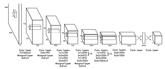
(détection d'objets dans les images)
---
## Fonctions de "loss"
On cherche à minimiser la perte, c'est-à-dire l'erreur entre $\mathbf{y}_i$ et $F_\mathbf{p}(\mathbf{x}_i)$.
$$
V(\mathbf{y}_i,F_\mathbf{p}(\mathbf{x}_i))=\|\mathbf{y}_i - F_\mathbf{p}(\mathbf{x}_i)\|^2 \quad\text{Très fréquent en approximation}
$$
Et on minimise sur toutes les données le risque empirique:
$$
Risk(F_\mathbf{p})=\frac{1}{N}\sum_{i=1}^{N}V(\mathbf{y}_i,F_\mathbf{p}(\mathbf{x}_i))
$$
:::info
Pour chercher les paramètres $\mathbf{p}$ qui minimise ce risque:
1) on part d'un choix $\mathbf{p}:=\mathbf{p}_0$ arbitraire
2) on modifie $\mathbf{p}$ progressivement pour que $Risk(F_\mathbf{p})$ diminue
Pour ce faire, on suit le **gradient** de $F$ par rapport à ces paramètres
:::
---
## Exemple: gradient d'un masque 3x1
Mettons $\left\lbrack\begin{array}{c}s_1 \\ s_2 \\ s_3 \end{array}\right\rbrack = F_\mathbf{p}\left( \left\lbrack\begin{array}{c}e_1 \\ e_2 \\ e_3 \end{array}\right\rbrack \right) = \left\lbrack\begin{array}{c}p_1 \\ p_2 \\ p_3 \end{array}\right\rbrack \ast \left\lbrack\begin{array}{c}e_1 \\ e_2 \\ e_3 \end{array}\right\rbrack = \left\lbrack\begin{array}{c} e_2 p_1+e_1 p_2 \\ e_3 p_1 + e_2 p_2 + e_1 p_3 \\ e_3 p_2 + e_2 p_3 \end{array}\right\rbrack$
Alors le gradient du risque peut s'écrire:
$\nabla_\mathbf{p} (Risk(F_\mathbf{p})) = \frac{1}{N}\sum_{i=1}^N \nabla_\mathbf{p}( \| \mathbf{y}_i - F_\mathbf{p}(\mathbf{x}_i)\|^2)$
Intéressons-nous juste au gradient pour la donnée $i$
$$
\left\lbrack\begin{array}{c}\frac{\partial}{\partial p_1} \\ \frac{\partial}{\partial p_2} \\ \frac{\partial}{\partial p_3} \end{array}\right\rbrack(\| \mathbf{y}_i - F_\mathbf{p}(\mathbf{x}_i)\|^2) = -2\left\lbrack\begin{array}{ccc}e_2 & e_3 & 0 \\ e_1 & e_2 & e_3 \\ 0 & e_1 & e_2 \end{array}\right\rbrack_{|\mathbf{x}_i} \cdot (\mathbf{y}_i - F_\mathbf{p}( \mathbf{x}_i))
$$
(On coupe les convolutions aux bords)
---
## Gradient des boites du réseau
:::success
La plupart sont faciles à calculer.
:::
* Couche ReLU: $\mathbf{s}=R(\mathbf{e})=\max(\mathbf{0},\mathbf{e})$, $R'(e_i)=1$ si $e_i \ge 0$, $0$ sinon
* Couche linéaire: $\mathbf{s}=R(\mathbf{e})=\mathbf{b}+\mathbf{W}\mathbf{e}$, $\nabla_\mathbf{e} R (\mathbf{e}) =\mathbf{W}$,
$\nabla_\mathbf{W} L(\mathbf{s}) = \nabla_\mathbf{s} L(\mathbf{s}) \mathbf{e}^T$, $\nabla_\mathbf{b} L(\mathbf{s}) = \nabla_\mathbf{s} L(\mathbf{s})$
* idem pour convolution, max-pooling, etc
---
## back-propagation I: réseau MLP et "forward pass"

$$
\begin{matrix}
\mathbf{f}_0=\beta_0+\Omega_0 \mathbf{x}_i & \mathbf{f}_1=\beta_1+\Omega_1 \mathbf{h}_1 & \mathbf{f}_2=\beta_2+\Omega_2 \mathbf{h}_2 & \mathbf{f}_3=\beta_3+\Omega_3 \mathbf{h}_3 \\
\mathbf{h}_1=\mathbf{a}[\mathbf{f}_0] & \mathbf{h}_2=\mathbf{a}[\mathbf{f}_1] & \mathbf{h}_3=\mathbf{a}[\mathbf{f}_2] & l_i=L[y_i,\mathbf{f}_3]
\end{matrix}
$$
---
### back-propagation II: "backward pass"

---
### back-propagation III: "backward pass"

:::success
On peut estimer l'influence des $\beta_k,\omega_k$ sur $l_i$ à partir des couches supérieures.
:::
$$
\begin{matrix}
\frac{\partial l_i}{\partial \mathbf{f}_3}=L'[y_i,\mathbf{f}_3] = 2(y_i-\mathbf{f}_3) \quad\text{(si moindres carrés)} \\
\frac{\partial l_i}{\partial \mathbf{\beta}_3} = \frac{\partial l_i}{\partial \mathbf{f}_3}, \quad \frac{\partial l_i}{\partial \mathbf{\Omega}_3} = \frac{\partial l_i}{\partial \mathbf{f}_3} \mathbf{h}_3^T, \quad \frac{\partial l_i}{\partial \mathbf{f}_2}=\mathbf{1}[\mathbf{f}_2 >0] \odot (\Omega_3^T \frac{\partial l_i}{\partial \mathbf{f}_3}) \quad\\
\frac{\partial l_i}{\partial \mathbf{\beta}_2} = \frac{\partial l_i}{\partial \mathbf{f}_2}, \quad \frac{\partial l_i}{\partial \mathbf{\Omega}_2} = \frac{\partial l_i}{\partial \mathbf{f}_2} \mathbf{h}_2^T, \quad \frac{\partial l_i}{\partial \mathbf{f}_1}=\mathbf{1}[\mathbf{f}_1 >0] \odot (\Omega_2^T \frac{\partial l_i}{\partial \mathbf{f}_2}) \ldots \\\end{matrix}
$$
---
## back-propagation du gradient
Si tous les composants de $F$ simple, on peut calculer symboliquement le gradient total
| In | Lin. 1 | Act. 1 | Lin. 2 | Act. 2 | ... | Lin. L | Act. L | Cost (train) |
|:------------:| ------------------------ | ------------------- | -------------------------- | ------------------- | --- | ------------------------------ | ------------------- | --- |
| $\mathbf{x}$ | $\mathbf{z}^1$ | $\mathbf{a}^1$ | $\mathbf{z}^2$ | $\mathbf{a}^2$ | | $\mathbf{z}^L$ | $\mathbf{a}^L$ | |
| | $\mathbf{W^1}\mathbf{x}$ | $f^1(\mathbf{z}^1)$ | $\mathbf{W^2}\mathbf{a}^1$ | $f^2(\mathbf{z}^2)$ | | $\mathbf{W^L}\mathbf{a}^{L-1}$ | $f^L(\mathbf{z}^L)$ | $C(\mathbf{y},\mathbf{a}^L)$ |
Erreur couche $L$, $\delta^L=(f^L)' \cdot \nabla_{\mathbf{a}^L} C=(f^L)' \cdot -2(\mathbf{y}-\mathbf{a}^L)$ (Err. quad.)
Erreur couche $L-1$, $\delta^{L-1}=(\mathbf{W}^L)^T \cdot \delta^L$
...
Gradient sur chaque poids: $\nabla_{\mathbf{W}^l}C=\delta^l (\mathbf{a}^{l-1})^T$