[CGDI] Geometry Processing: Laplacian smoothing and Tutte Embedding === > [name="David Coeurjolly"] ENS [CGDI](https://perso.liris.cnrs.fr/vincent.nivoliers/cgdi/) [TOC] --- In this practical, the objective is to play with basic mesh iterators/circulators either using the [geometry-central](https://geometry-central.net) (`c++`) or the [pygel3d](http://www2.compute.dtu.dk/projects/GEL/PyGEL/) (in `python`) APIs. # Warm-up 1. Read the last section of [this practical](https://codimd.math.cnrs.fr/s/4HjiHCH9z). 2. Get the code skeleton for this fourth practical (`git pull`) which corresponds to the last part of the third one (OBJ loading); compile or evaluate it. 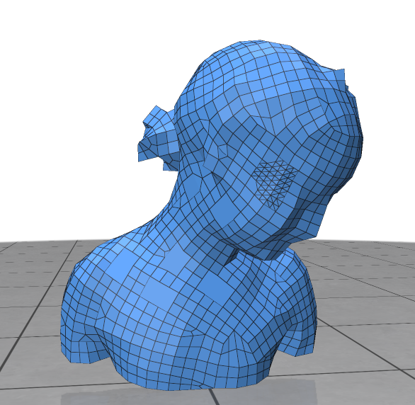At this point, you should be a able to visualize some [Wavefront OBJ files](https://en.wikipedia.org/wiki/Wavefront_.obj_file) (some examples are given in the folder `data/`). E.g. for `bimba-mix.obj`:  :::warning Questions 1 and 2 should take less than 10 minutes... If you get stuck for technical reasons, send us a message ASAP. ::: # Iterators, Circulators... In this practical, we will only consider meshes which are [discrete 2-manifolds](https://en.wikipedia.org/wiki/Surface_(topology)) (with boundaries). We won't go into the topological consequences of that statement but the basic properties are the following combinatorial ones: * The mesh has a graph structure $G(V,E)$ with vertices $V$ and edges $E$. * Faces are non-contractible cycles of $G$. * Each **interior** edge is adjacent to exactly two faces. Edges on the **boundary** are only adjacent to one face. * At each vertex, its adjacent faces define a topological disk. There are many libraries and utilities that load a mesh structure and provide the API and iterators to traverse the mesh. For instance, with [pygel3d](http://www2.compute.dtu.dk/projects/GEL/PyGEL/) and its [hmesh API](http://www2.compute.dtu.dk/projects/GEL/PyGEL/PyGEL/pygel3d/hmesh.html) ```python for f in mesh.faces: #do something on the face f for v in mesh.circulate_face(f): #do something on the vertex v of the face f ``` or ``` python for adjV in mesh.circulate_vertex(v, mode='v'): #... ``` to iterate over adjacent vertices to `v` (`mode='f'` will iterate over the adjacent faces and `mode='h'` over the adjacent halfedges). In [geometry-central](https://geometry-central.net) and its [surface_mesh navigation API](https://geometry-central.net/surface/surface_mesh/navigation/) it looks like: ``` c++ for(auto f: mesh.faces()) { #do something on the face f for(auto v: f.adjacentVertices()) #do something on the vertex v of the face f } ``` 3. Create a simple code that loads the `bimba-mix.obj` file and create a vertex quantity (cf previous practical) which contains to the degree at each vertex (i.e. number of adjacent vertices). 4. Create a simple OBJ debugger that prints a trace such as ``` face 0: has 4 vertices vertex 12 with coordinates (1.2,3.2,4.3) vertex 13 with coordinates (-1.2,3.2,1.3) vertex 22 with coordinates (1.2,13.2,.3) vertex 42 with coordinates (1.22,3.2,7.3) face 1: has 3 vertices .... ``` 5. Create a tool that scans the mesh and detect the vertices belonging to the boundaries of the mesh. `bimba-mix.obj` is a discrete 2-manifold without boundaries. To test your code, use `bunnyhead.obj`. :::warning To visualize such quantities, we encourage you to use the `polyscope` structures/quantities for *visual debugging*. For instance the output of the previous question could be a new point cloud containing the boundary vertices, as [count quantity](https://polyscope.run/structures/surface_mesh/count_quantities/) attached to the mesh vertices, or displaying the boundary edges as a [curve network](https://polyscope.run/structures/curve_network/basics/)... ::: # Laplacian and Taubin smoothing Being able to smooth a noisy geometrical object is one of the most fundamental geometry processing task. We would like you to implement one of the most elementary, yet efficient approach, is called the [Laplacian smoothing](https://en.wikipedia.org/wiki/Laplacian_smoothing). Let's start with the classical formulation (for $0<\lambda<1$): $$ v_{t+1} \leftarrow v_{t} + \lambda {L~}(v_t)$$ with $${L}(v_t)= \left(\sum_{v'\in\mathcal{N}(v_t)} \frac{v'}{|\mathcal{N}(v_t)|}\right) - v_t$$ AKA: Each vertex is displaced in the direction of its adjacent vertices barycenter with a step $\lambda$ ($\mathcal{N}(v)$ denotes the adjacent vertices to $v$). :::info This formulation refers to the *Laplacian* as the operator ${L~}$ is a rough finite difference approximation of the Laplacian operator applied to the mesh vertex positions. We will elaborate on that later. ::: {%youtube bFf9d-GyrR0 %} 6. Implement the Laplacian Smoothing. 7. If you consider an infinite number of steps (and no numerical issues), what shape is the fixed point of the Laplacian smoothing? What kind of *flow* does it imply? :::info As you may have guessed, the ${L~}$ operator can be replaced by more advanced discrete version of the [Laplace-Beltrami](https://en.wikipedia.org/wiki/Laplace–Beltrami_operator) operator such as the classical "cotan" one you have seen in the lecture: $$L(v_i) = \left(\frac{1}{\sum_{j\in\mathcal{N}(v_i)} w_{ij}} \sum_{j\in\mathcal{N}(v_t)} w_{ij} v_j\right) - v_i,\, \text{with}\,\, w_{ij}=\frac{1}{2}(cot \alpha_{ij} + cot \beta_{ij})$$ ::: Without spoiling the question 7, you may have observed that the Laplacian smoothing shrinks the surface. To fix that problem, Taubin[^1] has proposed a simple variation that iterates over the following two smoothing steps: $$ v_{t+1} \leftarrow v_{t} + \lambda {L}(v_t),\quad v_{t+2} \leftarrow v_{t+1} + \mu {L}(v_{t+1})$$ with a negative step $\mu$ such that: $0<\lambda< -\mu< 1$. The rationale behind the second step is to "inflate" the geometry in between to shrinking steps. | Original | Laplacian | Taubin | | -------- | 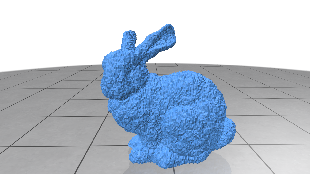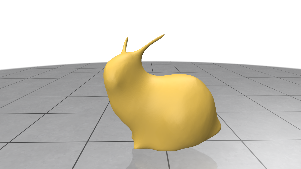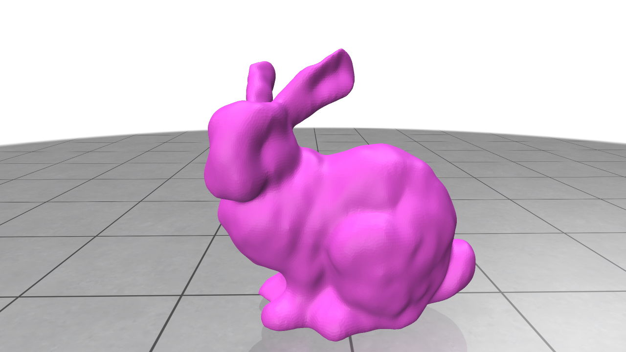-------- | -------- | |  |  |  | 8. **(extra)** Implement Taubin's approach. # Tutte Embedding Surface parametrization is a classical problem in the Computer Graphics in which you are looking for a new planar parametrization in $[0,1]^2$ of a generic mesh which minimizes a given distortion energy (*e.g.* area-preserving, angle-preserving --aka [conformal mapping](https://en.wikipedia.org/wiki/Conformal_map)--,...). As you may guess, such parametrization may not exist (*e.g.* rule surface for isometric mappings...) or may not be unique. Depending on the distortion model, we may have to consider approximated solutions. ::: info The distortion model is also tightly related to the topology of the input mesh. For instance, a conformal map exists for shapes homeomorphic to a disc but not for higher genius surfaces (embedded in Euclidean space). In that case, we may have to *cut-and-open* the surface, creating seams in the parametrization. 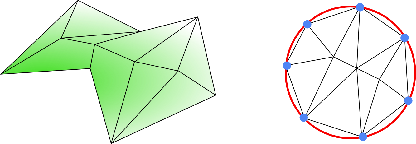::: A simple algorithm is given by the [Tutte Embedding](https://en.wikipedia.org/wiki/Tutte_embedding)[^2], first designed for planar graph embedding. For short, the algorithm exactly corresponds to the Laplacian smoothing approach: all **boundary vertices** are uniformly distributed on a unit circle and we smooth the interior vertices. 9. Using the code of the question 5 that tags vertices belonging to the boundary of a mesh, implement a first Tutte Embedding where the boundary vertices remain fixes. You can experiment it on the `bunyhead.obj` mesh (which is homeomorphic to a disk). At this point, you have solved a [Laplace's Equation](https://en.wikipedia.org/wiki/Laplace%27s_equation) with boundary conditions :+1: (not the most efficient way but still...). As the Tutte approach solves a Laplace problem, it is closely related to a conformal energy model. {%youtube GY_nc4P8u4g %} 10. Complete the parametrization task, distribute the boundary vertices regularly on a circle and perform the embedding of the interior vertices.  # References [^1]: Taubin, Gabriel. "Curve and surface smoothing without shrinkage." Proceedings of IEEE international conference on computer vision. IEEE, 1995. [^2]: Tutte, William Thomas. "How to draw a graph." Proceedings of the London Mathematical Society 3.1 (1963): 743-767.